1Department of Geosciences, University of Oslo, P.O. Box 1047 Blindern, 0316 Oslo, Norway
2Section for Glaciers, Ice and Snow, Hydrology Department, Norwegian Water Resources and Energy Directorate, P.O. Box 5091 Majorstua, 0301 Oslo, Norway
3Department of Earth Sciences, Uppsala University, Villav. 16, 752 36 Uppsala, Sweden
Correspondence:Andreas Kääb ([email protected]) Received: 7 July 2017 – Discussion started: 7 August 2017
Revised: 20 December 2017 – Accepted: 12 January 2018 – Published: 9 March 2018
Abstract.With dense SAR satellite data time series it is pos-sible to map surface and subsurface glacier properties that vary in time. On Sentinel-1A and RADARSAT-2 backscat-ter time series images over mainland Norway and Svalbard, we outline how to map glaciers using descriptive methods. We present five application scenarios. The first shows poten-tial for tracking transient snow lines with SAR backscatter time series and correlates with both optical satellite images (Sentinel-2A and Landsat 8) and equilibrium line altitudes derived from in situ surface mass balance data. In the sec-ond application scenario, time series representation of glacier facies corresponding to SAR glacier zones shows potential for a more accurate delineation of the zones and how they change in time. The third application scenario investigates the firn evolution using dense SAR backscatter time series together with a coupled energy balance and multilayer firn model. We find strong correlation between backscatter sig-nals with both the modeled firn air content and modeled wet-ness in the firn. In the fourth application scenario, we high-light how winter rain events can be detected in SAR time series, revealing important information about the area extent of internal accumulation. In the last application scenario, av-eraged summer SAR images were found to have potential in assisting the process of mapping glaciers outlines, especially in the presence of seasonal snow. Altogether we present ex-amples of how to map glaciers and to further understand glaciological processes using the existing and future massive amount of multi-sensor time series data.
1 Introduction
Glacier change is an important measure of the climate (Vaughan et al., 2013), and glaciers are therefore considered an essential climate variable (GCOS, 2003). Equable base-line datasets are fundamental for parametrization of models and in change analysis (e.g., Fontana et al., 2010; Winsvold et al., 2014; Huss and Hock, 2015) and are essential to better understanding the state of glaciers, especially in regions with scarce in situ observations.
Optical and synthetic aperture radar (SAR) satellite sys-tems for Earth observation have different advantages and dis-advantages for glacier observation. Many of the measured variables included in glacier change studies are often mapped using optical imagery (e.g., Racoviteanu et al., 2009). How-ever, the amount of images is limited in mountain, maritime and high-latitude regions due to cloud cover and the polar night. SAR instruments, in contrast, are largely insensitive to weather and, as active instruments, operate independent of solar radiation penetrating clouds. Using SAR and opti-cal imagery in combination should be of high value for un-derstanding processes and adding information for further ad-vances in glacier remote sensing applications (Kääb et al., 2014).
al., 2014). Together, these satellite sensors will enable new multi-sensor time series applications for mapping glaciers. In this work, we present continuous time series of Sentinel-1A SAR data (12-day repeat cycle) covering glaciers in Svalbard and mainland Norway. Since autumn 2016 two SAR sensors have been in orbit (Sentinel-1A and B), providing dense tem-poral sampling availability (6-day repeat).
Backscatter time series can detect changes in snow and ice conditions, which are related to the amount and variation of ice, air and water in the measured target (e.g., Forster et al., 1996). The received signals at the sensor reflect multi-ple scattering events dependent on SAR instrument frequen-cies, polarization and imaging geometry, as well as physical characteristics and dielectric properties of snow and ice (e.g., roughness, water content, grain size, temperature and impu-rities. Shi and Dozier, 1995; Lillesand et al., 2004; Wood-house, 2006). Backscatter signals show not only surface re-flectivity but also signals from below the surface (volume scattering), allowing for differentiation between SAR glacier zones (e.g., Fahnestock et al., 1993; Rau et al., 2000). Stud-ies since the 1980s have been used to investigate snow and ice, particularly using summer SAR images for exploring and tracking transient snow lines (TSLs) (Rott, 1984; Hall et al., 2000; Rees et al., 1995; Casey and Kelly, 2010; Callegari et al., 2016). Synergistic use of SAR and optical satellite im-agery for mapping snow and ice has been evolving since the 1990s (Rott and Strobl, 1992; Rott, 1994; Shi et al., 1994; Sephton et al., 1995). However, the use of dense continuous Sentinel-1A and B SAR backscatter time series has not been explored in this context.
In this paper, we present five application scenarios de-scribing new potential for mapping glaciers with dense high-resolution SAR satellite image time series based on robust methods. The chronological order of the imagery, or calcu-lated stack statistics of individual pixels or points (Winsvold et al., 2016), has been analyzed. (1) In the first application scenario, we have tracked the TSLs using SAR time se-ries data, and we describe the possible connection between TSLs from combined SAR–optical time series and equilib-rium line altitudes (ELA) from in situ surface mass bal-ance (SMB) measurements. (2) Second, we show the stabil-ity of winter backscatter values and the potential of observing glacier facies from 2009 to 2016 using both Sentinel-1A and RADARSAT-2 SAR-data. (3) Third, SAR time series of sur-face and subsursur-face observations have been compared with a SMB and firn evolution model (Van Pelt and Kohler, 2015) using glacier centerlines profiles. (4) Fourth, we show the potential to map winter rain events over glaciers using high temporal resolution SAR backscatter data. (5) Fifth, we have investigated patterns in summer SAR backscatter signals on-and off-glacier on-and their potential in glacier outline mapping. For each individual application scenario, a brief introduction, background and method part is given, and results are pre-sented and discussed.
2 Study areas
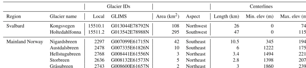
In this paper, we have studied two glaciers near Ny-Ålesund on Svalbard (78.8◦N, 12.7◦E) and five glaciers in south-ern Norway (61–62◦N, 7–8.6◦E; Fig. 1 and Table 1). An-nual mean temperature for Ny-Ålesund is−5.7◦C, and mean winter and summer temperatures are−12.9 and 3.7◦C, re-spectively (normal period 1971–2000; Isaksen et al., 2016). Glaciers on Svalbard are maritime and often have a superim-posed ice zone (Hagen et al., 2003). Superimsuperim-posed ice forms from meltwater or rain that refreezes at the surface of the ice (Cogley et al., 2011). Kongsvegen (108 km2)surged in 1948 (Melvold and Hagen, 1998) and is currently in its quiescent phase with low flow velocities (Nuth et al., 2012). Krone-breen, the lower part of Holtedahlfonna (together 295 km2), is a fast-flowing tidewater glacier with maximum ice veloc-ity of 3.2 m d−1at the calving front (Schellenberger et al., 2015).
In southern Norway, the five studied glaciers form a maritime–continental transect and represent diverse glacier characteristics. Nigardsbreen (42 km2) and Austdalsbreen (10 km2)are outlet glaciers from the ice cap Jostedalsbreen. Storbreen (5 km2), Hellstugubreen (3 km2)and Gråsubreen (2 km2)are smaller valley glaciers located in the high moun-tain area of Jotunheimen. Due to the elevation and more east-ward location, these glaciers are more continental than Ni-gardsbreen and Austdalsbreen. For Norwegian glaciers, the superimposed ice zone is usually absent, even though it may be present on some glaciers (e.g., Brown et al., 2005). The glaciers in mainland Norway all have SMB programs mea-sured by the Norwegian Water Resources and Energy Direc-torate (Kjøllmoen et al., 2017).
3 Satellite data
Time series from two SAR sensor types were used in this study, namely Sentinel-1A and B (Interferometric Wide swath mode, IW) and RADARSAT-2 (Wide, Wide Fine and ScanSAR-Wide modes) (Table 2). Both SAR sensor types acquire in C-band (center frequency of 5.405 GHz and wave-length of 5.5 cm), and images are single polarized SAR data (HH for Svalbard and VV for mainland Norway). Sentinel-1A and B orbits for mainland Norway and Sentinel-Sentinel-1A for Svalbard are ascending and right looking. Some data gaps ex-ist due to missing images in the download archive (Sentinel-1A) or due to limitations of the data quota and priority (RADARSAT-2).
100 m. The images were acquired from different incidence angles and either ascending or descending paths.
Optical satellite data have been included for validation purposes, though with lower temporal resolution mostly due to extended cloud cover in the maritime study regions. Medium-resolution optical satellite imagery, Landsat 8 OLI (level 1 terrain) and Sentinel-2 MSI (level 1C), was avail-able with radiometrical corrected and orthorectified products (Dursch et al., 2012; Roy et al., 2014). These were used for comparison with SAR imagery in the snow line tracking application from Hellstugubreen and Kongsvegen (Sect. 5.1 and Table A2). High mountain areas in mainland Norway are often highly affected by cloud cover, and only six im-ages were usable for comparison with SAR (three in 2015 and three in 2016). For Kongsvegen on Svalbard, nine opti-cal images were used (five in 2015 and four in 2016). The dates of the optical imagery correlated with the SAR acqui-sitions by±3 days, with two exceptions having a 6-day gap (Table A2). In addition, a Landsat 8 image from 11 Septem-ber 2015, corresponding to day of year (DOY) 254, was used in the glacier outline mapping (Sect. 5.5).
3.1 Additional data
Interpretation of SAR backscatter images for glacier map-ping purposes can be challenging since several factors and processes on and within the subsurface affect the phase and magnitude of the SAR signals. The snow, firn and ice are dependent on external and surface conditions and can result in similar backscatter values. Therefore, additional data, or comparison datasets, were used to check the quality and reli-ability of the SAR time series. Meteorological data, temper-ature and precipitation, were downloaded from the Norwe-gian Meteorological Institute (eKlima.no, 2016) for the Ny-Ålesund meteorological station (Svalbard) and Juvvasshøe meteorological station (mainland Norway) (Figs. A1 and A2). Both stations are located close to the three glaciers used for detailed analysis of the backscatter time series, namely Hellstugubreen (within ∼12 km and station is lo-cated 1894 m a.s.l.), Kongsvegen and Holtedahlfonna (within ∼20 km and station is located 8 m a.s.l.). We have used ex-isting glacier outlines from both Svalbard (Nuth et al., 2013)
Figure 1.Study area in Svalbard (local IDs: 15511.2 is Holtedahl-fonna and 15510.1 is Kongsvegen) and southern Norway (local IDs: 2478 is Austdalsbreen, 2297 is Nigardsbreen, 2636 is Storbreen, 2768 is Hellstugubreen and 2743 is Gråsubreen) (Glacier outlines from Nuth et al., 2013; Andreassen et al., 2008; Paul et al., 2011).
and mainland Norway (Andreassen et al., 2008; Paul et al., 2011) as verification and in support of the analysis. Updated glacier outlines for the Norwegian glaciers are available (An-dreassen et al., 2016). The discrepancies between new and old outlines are minor and do not influence the results pre-sented in this paper.
4 Processing of SAR imagery
Figure 2.A heat plot of Sentinel-1A backscatter (dB) time series from 22 January 2015 to 13 September 2016 (DOY 22 2015 to 257 2016), along a profile on Kongsvegen, Svalbard. It is 12 days between each Sentinel-1 acquisition. The numbers represent 11 possible glacier mapping variables that can be detected from the SAR time series: (1) onset of cold season; (2) freeze-up and evolution of the firn area as the winter cold wave penetrates the snow and firn; (3) winter rain event; (4) change of surface properties after winter rain event; (5) glacier facies, separated by firn line altitude (FLA) and superimposed ice altitude (SIA) (SI is superimposed ice); (6) onset of melt season; (7) transient snow lines (TSL); (8) end of summer snow line (EOSS); an estimation of the equilibrium line altitude (ELA); (9) length of melt season; (10) surface dry-to-wet snow line; and (11) glacier outline or calving front. The two sketches above the heat plot represent the SAR glacier zones in the cold season (winter with dry and cold conditions; snowpack is transparent due to high volume scattering) and in the melt season (summer with warm and wet conditions), together representing a full mass balance year. (Illustration insets above the heat plot are modified based on de Ruyter de Wildt et al., 2002.)
The Sentinel-1A and B GRD images were in slant range co-ordinates projected to an ellipsoid, and RADARSAT-2 single look complex images were in radar geometry. The Sentinel-1 images in SNAP were converted to radiometrically cali-brated backscatter in sigma nought (σ0)and then filtered us-ing a 3×3 median speckle filter. Furthermore, we applied backscatter terrain correction using a digital elevation model (DEM) and converted linear backscatter values to decibels (dB). The radar backscatter coefficient (σdB0 ) is hereafter referred to as backscatter. To examine the backscatter re-sults produced in SNAP, we tested the difference between GAMMA and SNAP processed Sentinel-1A GRD images for two winter dates over the glaciers of interest. In GAMMA, the radiometric calibration corrects for two effects: (1) the varying incidence angle on the returned backscatter and (2) the differing pixel illumination that depends upon the in-cidence angles (resulting in gamma nought,γ0). A speckle filter was not applied on the Sentinel-1 and RADARSAT-2 images in GAMMA. However, a multi-look algorithm was applied to reduce noise using spatial averaging. In
T able 2. Ov ervie w of Sentinel-1A and B and RAD ARSA T -2 data. aRAD ARSA T -2 images are in W ide (2009–2013) and W ide Fine (2014–2015). here, as only fi v e images within 8 days were used as ancillary data. bGRD: ground-range-detected images ha v e been detected, multi-look ed using an ellipsoid (WGS84). cSentinel-1B ima ges were av ailable in mainland Norw ay since 3 October 2016 (DO Y 277). Some Sentinel-1A from the Sentinels Scientific Data Hub and ha v e caused acquisition g aps in the time series. F or RAD ARSA T -2 the time g aps are due to (Abbre viations: θi is incident angle, Pol. is polarization, T emp.res. is temporal resolution, Rel. path is the relati v e path, and Da ta prod. is data RAD ARSA T -2 a Sentinel-1A and Glacier re gion No. Pol. θi Start date End date T emp. res. No. Pol. Rel. path Start date End date Sv albard 63 HH 37.8 ◦ 8 Feb 2009 17 Dec 2015 24 days 37 HH 14 22 Jan 2015 13 Sep Mainland Norw ay – – – – – – 51 VV 44 20 Oct 2014 15
Oct al., 2016). A sufficient geocoding and co-registration ensures
that the pixels can be compared in time.
A dense satellite image time series provides the opportu-nity to recover a large statistical sample of backscatter values. Heat plots were used for visual inspection of the temporal signature of the glaciers: along the centerline, profile points were selected every 300 m for the Svalbard glaciers (Fig. 2) and by calculating the mean backscatter value in elevation zones of 25 m. The latter was applied on the study glaciers in mainland Norway (Fig. 3a). Backscattering intensity values are normally very noisy, and the data from the profiles were smoothed using the mean of 7×7 pixel values (30 m pixel size). Representing SAR backscatter data in such a way, we present 11 different mapping variables from the SAR time series illustrated by numbers on the Kongsvegen profile in Fig. 2.
5 Application scenarios
In this section we present application scenarios using SAR time series dataset for glacier mapping and discuss the re-sults.
5.1 Seasonal melt patterns
The amount of usable images for reconstruction of annual mass balance based on EOSS is more predictable with SAR imagery compared to using optical satellite data due to a reli-able repeat passes of the Sentinel-1 satellites and transparent clouds.
Wet snow absorbs most of the microwave signal, returning little energy back to the sensor (Stiles and Ulaby, 1980). The roughness of snow or ice and incidence angle of the SAR satellite sensor also affects the backscatter signal strength (Shi and Dozier, 1995, Fig. 4). In both the Sentinel-1A and RADARSAT-2 backscatter time series an abrupt seasonal change was found, from warm and wet conditions in the end of the melt season to the onset of the cold season with dry and cold conditions (corresponding to no.1 in Fig. 2). These backscatter differences are present due to a change in weather conditions between 26 August 2015 (DOY 238) and 7 September 2015 (DOY 250), causing an increase of∼ −20 to∼ −7 dB (Fig. 2). A temperature record from the closest weather station in Ny-Ålesund (8 m a.s.l.) shows lower tem-perature in the period between the images, indicating even colder temperatures on the glaciers since they are located on higher elevation (Fig. A2). In addition, an optical image from 9 September 2015 (DOY 252) over Kongsvegen shows sig-nificant precipitation as snow (Table A2), which also indi-cates conditions<0◦C on the glacier. The snow line, where the onset of cold season starts, corresponds to number 8 in Fig. 2, representing the EOSS. The onset of surface melt is characterized by a rapid decrease in backscatter values (cor-responding to no. 6 in Fig. 2; Stiles and Ulaby, 1980; Smith et al., 1997; Wolken et al., 2009), most likely introduced by warm and wet weather conditions (Rotschky et al., 2011). The lowest backscatter values in the ablation zone are found when wet snow covers the glacier (corresponding to no. 9 and the blue color in Fig. 2), which also reflects the length of the melt season. This has until now been mostly studied us-ing QuikSCAT data (a Ku-band sensor) with daily temporal resolution, but low spatial resolution (e.g., Rotschky et al., 2011). It is difficult to define the melt season accurately in time from RADARSAT-2 images due to the low repeat time of 24 days (Fig. 5). Sentinel-1 provides 6-day repeat time with two satellite sensors and can be used to study the length of the melt season more accurately in terms of spatiotempo-ral resolution.
The TSL migration up-glacier is often correlated with tem-perature rise and topography (e.g., Hall et al., 2000; corre-sponding to no.7 in Fig. 2). It is also possible to track the wetness in the snow up-glacier with the surface dry-to-wet seasonal snow line (corresponding to no. 10 in Fig. 2), but here we have focused on the TSL. During the melt season, seasonal snow melts away exposing a rough ice or firn sur-face, thus creating a sharp contrast to the smooth and wet snow. Based on similar observations by Hall et al. (2000), we believe this can be observed from SAR backscatter due to different roughness lengths between the two targets caus-ing higher scattercaus-ing of the ice surface (Fig. 4). We have used
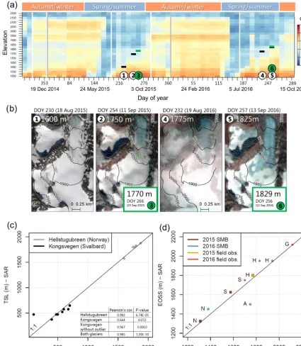
this difference in roughness to track the TSL within the melt season. When tracking the TSLs within a melt season, the few optical images available can be gap-filled with SAR data (Fig. 3a, b). TSLs from optical and SAR images acquired almost on the same day were manually selected from the glaciers (Table A2). Heat plots, a DEM, SAR backscatter and optical satellite images were used for visual inspection of the TSL positions in the analysis (see also temperature plot in Fig. A1). Using mean backscatter in elevation zones of 25 m gives a location of the TSL representing the width of the glacier compared to using a centerline representing one point on the glacier. The same visual interpretation was used to retrieve the EOSS from SAR acquisitions on four of the glaciers in 2015 and 2016 (Hellstugubreen, Storbreen, Ni-gardsbreen and Austdalsbreen). On Gråsubreen we detected a melt regime which did not correlate with elevation, as the snowmelt was first apparent in the convex areas higher up on the glacier and not in the lower part where the snow accumu-lates (most likely due to the local topography and wind pat-terns). On such glaciers, satellite sensors other than Sentinel-1A and B and their according dense time series are not able to reveal the same level of temporal detail in melt patterns.
Strong correlation was found between TSLs from Sentinel-2 and Landsat 8 satellite images and TSLs from Sentinel-1 images (Fig. 3a, b, c). In the melt season with warm and wet conditions, the backscatter signal after snow events might be reduced on the glacier. They can cause, firstly, a smoother surface compared to the underlying rougher ice surface and, secondly, high absorption and for-ward scatter of the radar waves as the snow is wet (Rott, 1984). An example of this was when lower backscatter val-ues were observed in the ablation area of Hellstugubreen on 3 October 2016 (DOY 277), most likely due to wet snow lowering the roughness and absorbing microwave energy (Fig. 3a). Snow was observed in an optical image on 6 Oc-tober 2016 (DOY 280) on Hellstugubreen (not shown). In addition, another example from Kongsvegen showed a snow event causing disagreement between the Landsat 8 image and Sentinel-1 images (see outlier in Fig. 4c). This snow event must have happened between the compared acquisition dates of the optical and SAR satellite images (i.e., between 7 and 9 September 2015, DOY 250 to 252; Table A2).
Figure 4.Photos illustrating roughness differences between ice or firn and seasonal snow. The images of Hellstugubreen were acquired on 12 September 2016 (DOY 256), when the end of summer snow line can be observed, often corresponding to the ELA (corresponding to no.8 in Fig. 2). Photos: Liss M. Andreassen, NVE.
ELA was “above” the glacier (ELA from SMB in 2016 was
>1747). The maximum discrepancy between a field obser-vation and a SAR acquisition was 21 days (SAR acquisition 3 October 2016 (DOY 277) and in situ on 12 September 2016 (DOY 256) on Hellstugubreen) (Fig. 3d).
In both study regions, we found a discrepancy between the datasets in that the TSLs from SAR generally show a mean of 21 m lower altitude compared to optically derived TSLs (not taking the outlier into consideration; Fig. 3c). On Kongsve-gen, as the snow line retreats up into the superimposed ice or firn area, the roughness difference is less compared with glacier ice, making it more difficult to retrieve a correct TSL (Figs. 5 and 6a). The same applies to optical satellite images as it is challenging to derive the TSL when superimposed ice is present (e.g., Winther, 1993; Kundu and Chakraborty, 2015).
The glacier geometry, elevation, size, sun exposure and lo-cal snow accumulation influence the melt pattern of seasonal snow on glaciers, and thus the EOSS. If the glacier spans a small elevation range, the TSL could be more difficult to trace and may be either above or below the elevation range that the glacier covers. In addition, interaction between snow lines and crevassed areas, especially in ice falls, can be a challenge on larger glaciers (e.g., Chinn, 1995). Extracting TSLs and EOSS using SAR backscatter data can be valuable for
1. refining spatial variations in the melt pattern of well-studied glaciers with already existing surface mass bal-ance programs;
2. including many glaciers in the analysis, if the purpose is to derive the TSL and EOSS from SAR imagery to reconstruct annual mass balance series regionally and retrieve a statistical robust result;
3. using TSLs and EOSS for calibration and validation of mass balance models (e.g., Hulth et al., 2013).
5.2 Identifying glacier facies
Figure 5.RADARSAT-2 time series of SAR backscatter values (dB) along a centerline profile on Kongsvegen from 2009 to 2015. An abrupt change in the start and end of melting season (e.g., in year 2012 and 2013) was observed. The backscattering values are in decibel (dB).
In this application scenario, we present a time se-ries of SAR glacier zones from 2009 to 2016 including RADARSAT-2 (24-day repeat) and Sentinel-1A (12-day re-peat) images in northwest Svalbard. Previous studies have correlated distinct glacier facies with SAR glacier zones on Kongsvegen (Engeset et al., 2002; König et al., 2004; Brandt et al., 2008; Langley et al., 2008), and these facies also corre-spond to previous interpretations in literature (Benson, 1962; Rau et al., 2000; Cuffey and Paterson, 2010). Dry-snow glacier facies is absent on both Kongsvegen and Holtedahl-fonna as melting occurs over the entire surface (Engeset et al., 2002; Langley et al., 2007), which agrees with our inter-pretation of the SAR backscatter time series (Fig. 2). The firn line does not vary much from year to year, but several years of negative mass balance will eventually migrate the firn line up-glacier, and vice versa with positive mass balance years (e.g., König et al., 2004; Brown, 2012). Wet snow typically has the lowest backscatter values, followed by wet and dry ice (here, these show similar values; Fig. 2), dry superim-posed ice and dry snow and firn (Fahnestock et al., 1993). A dry-snow pack has low dielectric contrast, and SAR mi-crowaves are volume scattered. In the firn area, ice lenses, pipes and layers act as randomly oriented dielectric cylin-ders, responsible for the high scattering of microwave signal back to the SAR sensor. We consider snow and firn to be Rayleigh scatterers when the particle size is lower than 10 % of the wavelength (λ=5.5 cm) or 0.55 cm and Mie scatter-ers up to 10 times the wavelength, or 55 cm (Woodhouse, 2006). The backscatter response of superimposed ice is de-pendent on air bubble content and size, where a high fre-quency of bubbles typically causes higher backscatter values (e.g., König et al., 2002; Langley et al., 2009). Thus, dur-ing the cold season, the superimposed ice zone has typically lower backscatter compared to firn, but higher than glacier
ice (e.g., Langley et al., 2009). During the melt season, high backscatter on ice surfaces is caused by surface roughness rather than volume scattering (Shi and Dozier, 1995; Hall et al., 2000).
Figure 6.Observed backscatter and modeled values along the Kongsvegen centerline profile.(a)Sentinel-1A backscatter (dB) time series from 22 January 2015 to 13 September 2016 (DOY 22 2015 to 257 2016). (b) Modeled firn air content in a vertical column of 2 m;
(c)Spearman correlation between the firn air content (in panelb) and backscatter values (in panela) along the centerline for each Sentinel-1A acquisition time (each 300 m point). Significant correlation values (after Bonferroni multiple testing correction) are shown in red. Points on the black stippled line corresponds to missing data (white areas in panela).
the root-mean-square (RMS) surface height variation is more than 1.3 cm and considered a smooth surface when the RMS height variation is less than 0.2 cm (Lillesand et al., 2004). Drying of meltwater channels does not cause the backscatter to be higher in the cold season compared to the melt sea-son because they cover only a very small percentage of the SAR pixels; therefore we believe the ablation effect (caused
by melting and water on the ice surface) is responsible for a rougher surface and higher backscatter.
indicat-In this example, we show the potential to detect and study changes in transient glacier facies. Here, a stabilization of the SAR glacier zones in the cold season improves certainty about the designation of glacier facies.
5.3 Firn evolution and internal processes
For the first time, we present a comparison of Sentinel-1A backscatter time series with results from a SMB and firn pack evolution model. A coupled energy balance–multilayer firn model was used to simulate the evolution of tempera-ture, density and water content in snow and firn. The model has previously been used to simulate the long-term (1961– 2012) mass balance and firn evolution of Kongsvegen and Holtedahlfonna, as described in Van Pelt and Kohler (2015). For the experiment in this paper the model is forced with weather station data from the Ny-Ålesund weather station (provided by the Norwegian Meteorological Institute), which provided time series at sea level for temperature, precipi-tation, relative humidity, cloud cover and air pressure. El-evation lapse rates for temperature and precipitation were optimized to remove biases between modeled and observed seasonal mass balance. The precipitation lapse rate was optimized against winter balance data, and the tempera-ture lapse rate was optimized against summer balance data. Lapse rates were determined individually for Kongsvegen and Holtedahlfonna, which is mainly relevant for precipita-tion, which is known to increase much faster with elevation on Kongsvegen than on Holtedahlfonna (Nuth et al., 2012). Validation of modeled subsurface density against shallow firn core observations on Kongsvegen and Holtedahlfonna has been discussed in Van Pelt and Kohler (2015), showing good agreement. There is no real validation for subsurface temperature and water content for these glaciers. However, the model performed well in simulating vertical tempera-tures at the top of Lomonosovfonna, as shown in Van Pelt et al. (2014). Model output contains daily depth-dependent fields with a 300 m horizontal spacing along centerline pro-files on the glaciers. The sub-surface grid contains a total of 100 layers with layer thickness increasing with depth and ranging between 10 and 40 cm. Here, firn air content and the subsurface water content were compared with the SAR
by seasonal snow had low firn air content (e.g., at 7 Septem-ber 2015, DOY 250 in Fig. 6b). During the cold season the firn air content increased through time and moving up-glacier, as fresh snow accumulated (e.g., at 23 April 2016, DOY 113 in Fig. 6b). We observed high backscatter values (Fig. 6a) when firn air content was high (Fig. 6b), as the dry and cold conditions were found to enhance volume scatter-ing. For each Sentinel-1A acquisition, we found a positive significant correlation between firn air content and backscat-ter in the cold season and a negative significant correlation in the melt season (Fig. 6c). To avoid assumptions of a lin-ear relationship between firn air content and backscatter, we used the nonparametric Spearman’s rank correlation coeffi-cient. The reason for the negative correlation is the change of surface properties affecting the backscatter signal, as the volume scattering in the cold season is exchanged with the SAR sensitivity to wet snow and higher surface roughness in the melt season. The point in Fig. 6c on 1 September 2016 (DOY 245) showed no correlation, because it is located in the transition zone between the melt season and cold season, where multiple melt end freeze events happen within short time spans. The snow line was identified in the modeled data (Fig. 6b) and in the observed backscatter data (Sect. 5.1).
Figure 7.The figures show results from Holtedahlfonna(a)Sentinel-1A SAR backscatter (dB) time series from 22 January 2015 to 13 September 2016 (DOY 22 2015 to 257 2016). Black points indicate where the backscatter stabilizes in the cold season.(b)Daily modeled water content for each 300 m point along a centerline profile and the transition depth (in meters) between wet snow and firn (water con-tent>0) and dry snow and firn (water content=0). The white regions in the plot indicate no water since it is glacier ice with no snow in the summer or with dry-snow conditions in the winter. Transition depth of 0 m indicates wet-snow conditions on the surface.(c)Spearman correlation between depth of dry-to-wet transition zone and backscatter values plotted with elevation (yaxis) in firn area above 775 m. We used a time period with stable conditions: 7 September 2015 to 22 April 2016 (DOY 250 2015 to 113 2016; black box in panelsaandb). Sig-nificant correlation values (after Bonferroni multiple testing correction) are plotted in red.(d)Plot of backscatter values (dB) vs. dry-to-wet transition depth (layer) for points in(c)withpvalue>0.05 (points under∼920 m, using the same time period of 7 September 2015 to 22 April 2016, DOY 250 2015 to 113 2016). The correlation coefficients are 0.266 (Pearson’s correlation coefficient) and 0.3 (Spearman rho).
The backscatter measured at the sensor antenna is the sum of multiple scattering occurrences throughout the firn volume. The penetration depth of radar waves varies over time and contributes to the backscatter, and the backscatter intensity is therefore not constant in time and represents the integral of depth through time. Using the modeled data, we were able to explore the penetration of SAR backscatter in snow and firn. It is likely that absorption with limited volume scattering of radar waves in wet snow and firn can give an indication of how deep the Sentinel-1A C-band SAR can penetrate due to a strong sensitivity to wet conditions. Using the model re-sults we were able to estimate the depths of the intersection between the dry and wet zone in the firn pack (Fig. 7b) and compare this to the backscatter data (Fig. 7c–e). Results in-dicate increased penetration depths over time and then stabi-lization once the transition exceeds a certain depth where the radar waves do not reach it anymore. Similar trends between the transient modeled dry-to-wet transition depth in the firn and the backscatter time series for the uppermost part of the glacier were found (Fig. 7c). The deeper the dry-to-wet tran-sition zone, the higher the SAR backscatter values (Fig. 7e). This correlation can thus be explained by a mix of volume scattering returns and radar waves sensitivity to wet condi-tions in snow and firn through time until January 2016.
To investigate the penetration depth further, values from black points in Fig. 7a were selected where the backscat-ter values stabilized in the firn. Values from the same points of dry-to-wet transition depths (Fig. 7b) gave an indication of the depth of the dry-to-wet zone in the backscatter data. The mean transition depth of the point values from Fig. 7b is 1.7 m when all nine points were included. When only includ-ing the upper six points with significant correlation>920 m (showed in Fig. 7c and e), a mean transition depth of 2.0 m was found. We speculate that backscatter intensity cannot re-flect small changes in snow depth during the dry wintertime due to high volume scattering, thus suggesting deeper and temporally constant penetration of the radar waves.
In this example, modeled data were used to help interpret time series of backscatter intensity data. This might be in-verted in the future, as SAR backscatter data will be further understood and can potentially be used as refined model-ing input. Such information is valuable in remote regions in
glaciological context as it can be a substantial component to internal accumulation as it refreezes in the snow pack (e.g., Jansson et al., 2003; Van Pelt and Kohler, 2015; Van Pelt et al., 2016). The SAR backscatter contrast of ice and snow is directly dependent on the meteorological conditions be-fore and at the time of acquisition of the satellite image. Rain on an ice surface gives stable backscatter values sim-ilar to dry ice, since glacier ice is still rough even when wet. Consequently, roughness is considered as a highly impor-tant scattering variable (e.g., Hall et al., 2000). Wet snow absorbs SAR waves, and little energy is transmitted back to the SAR sensor in comparison to dry snow and firn surfaces (Rott, 1984). During dry-snow conditions, the radar signals depend on the underlying firn or ice conditions (e.g., Brown et al., 2005). In this application scenario, we have examined a rain event on Kongsvegen and Holtedahlfonna from dense Sentinel-1A images during the cold season (corresponding to no. 3 in Fig. 2; see time series animation of Kongsvegen in Supplement). RADARSAT-2 ScanSAR satellite images were used to investigate the extent of the rain event.
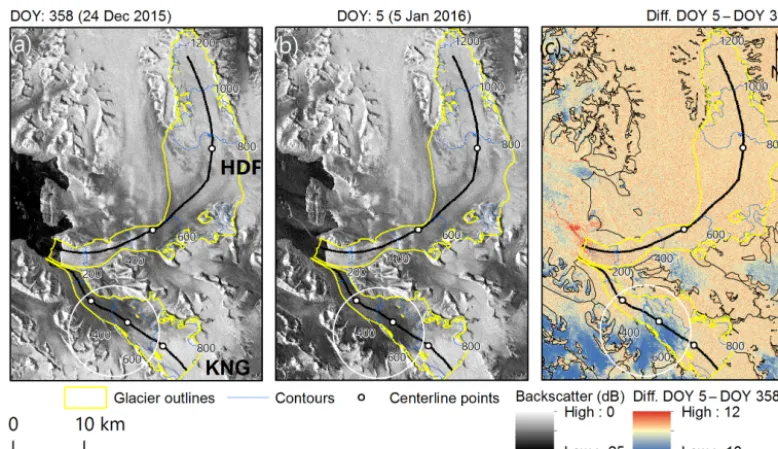
On 5 January 2016 (DOY 5), Sentinel-1A acquired an im-age over the Kongsfjorden region indicating wet conditions on the upper part of Kongsvegen and its surroundings (cor-responding to no. 3 in Fig. 2). The temperature and pre-cipitation data from Ny-Ålesund showed a warm and wet weather event from 29 December 2015 (DOY 363) to 4 Jan-uary 2016 (DOY 4) (Fig. A2 and Table A1). Figure 8a and b show backscatter images before and after the rain event, and Fig. 8c, which shows the difference between the two, in-dicates an area of wet conditions (blue color). Presumably, the extent of the rain event covered the entire surface of Kongsvegen. However, on the lower part on the glacier (the ice facies) this was hard to observe due to little snow and rough surface. A clearer signal was found further up-glacier with present seasonal snow on firn (white circle in Fig. 8b).
Figure 8. (a)Sentinel-1A backscatter (dB) image from 24 December 2015 (DOY 358) and(b)the following Sentinel-1A backscatter image from 5 January 2016 (DOY 5) showing remnants of the rain event.(c)The difference between 5 January 2016 (DOY 5) and 24 December 2015 (DOY 358) SAR intensity images. Blue color indicates a lowering of backscatter values between the images, showing wetter conditions in the upper firn of Kongsvegen (white circles). Glacier outlines from 2007 (Nuth et al., 2013).
and Table A1), colder conditions were measured on 4 Jan-uary 2016 (DOY 4, 1 day before the Sentinel-1A acquisi-tion). As stable low backscatter values were observed on 4– 5 January 2016 (DOY 4 to 5) (Fig. 9 and Table A1), we sug-gest that capillary water in the snow and firn, which was not yet frozen, was detected by the Sentinel-1 image on 5 Jan-uary 2016 (DOY 5). This could be related to the isolation capability of snow and release of latent heat when water re-freezes.
The same wet-snow conditions were not found on Holtedahlfonna (Figs. 7a and 8c). We observed a rain event on Holtedahlfonna on 30 December 2015 (white arrow on DOY 364 in Fig. 9), corresponding to 26.5 mm rain in Ny-Ålesund (Table A1). In the following days, Holtedahl-fonna had gradually higher SAR backscatter values, while Kongsvegen remained dark (low backscatter). Either pre-cipitation fell as snow on Holtedahlfonna between 3 and 5 January 2016 (DOY 3 to 5) or conditions were cold with no snowfall. Thus, the RADARSAT-2 ScanSAR images re-vealed different local weather conditions in the Kongsfjor-den region. Colder conditions are in general present on Holtedahlfonna as it has a more continental climate com-pared to Kongsvegen, indicating that the rainwater in the snow and firn pack froze faster than on Kongsvegen.
Directly after the winter rain event, we observed a chang-ing backscatter pattern in the ablation zone and lower part of the superimposed ice zone, indicating change in snow and ice properties on Kongsvegen (corresponding to no. 4 in Fig. 2). A change was also apparent from the modeled firn air content in Fig. 6b and reflects an increase in air content in the snow
and firn pack after a rain event. Backscatter values increased
>2 dB after the winter rain event between 300 and 600 m, and the border between the superimposed ice and ablation zone became unclear (Fig. 6a). We know from in situ obser-vations on Kongsvegen that glacier ice in the ablation area was covered with little snow in the spring 2016. The lower zone of the ablation area might have had little snow cover already before the rain event since the backscatter was con-tinuously low during winter (indicated by light blue color in Fig. 6a; present around the 200 m elevation line from 17 Jan-uary to 4 May 2016, DOY 17 to DOY 125). In the upper zone of the ablation area and before the rain event, more snow was present compared to lower elevations. Ice lenses and pipes might thus have been created from this penetration of water in the snow after the rain event, resulting in snow saturation giving stronger permittivity contrast as shown by increasing backscatter values (indicated by yellow color in Fig. 6a; present around the 400 m elevation line from 17 Jan-uary to 4 May 2016, DOY 17 to DOY 125).
Detection of winter rain events from SAR time series might be used to refine modeling inputs, especially in regions where meteorological data are scarce.
dif-Figure 9.RADARSAT-2 ScanSAR mode backscatter (dB) images from 29 to 30 December 2015 (DOY 363 and 364) and 3–5 January 2016 (DOY 3 to 5). Conditions on Holtedahlfonna were wet on 30 December (see white arrows) but were dry and cold again on 3–5 January 2016 (DOY 3 to 5) (higher backscatter than on 30 December 2015 (DOY 364). Low backscatter values were found on Kongsvegen from 3 to 5 January 2016 (DOY 3 to 5; see red arrows), indicating wetter conditions and more rainfall in this period compared to Holtedahlfonna.
ficult to separate seasonal snow from glacier and perennial snow patches (e.g., Andreassen et al., 2012; Winsvold et al., 2016). Local differences in weather conditions within a sin-gle optical satellite scene are common in high mountain re-gions. Mapping conditions in a single optical image might not be ideal due to cloud cover, seasonal snow around the glacier perimeter and thin layers of newly fallen snow. In-terferometric coherence images have been used for deriving glacier outlines (e.g., Atwood et al., 2010; Falk et al., 2016). In maritime regions such as southwestern Norway it can be challenging to use SAR coherence images due to rapid co-herence loss between the time of acquisitions often caused by precipitation, melt and wind. SAR backscatter informa-tion can be a valuable replacement. Wet snow and ice sur-faces have lower backscatter values than a snow-free surface outside the glacier (Rott, 1984; Strozzi et al., 1997). In this application scenario, we investigate how averaged summer SAR images from glaciers in southern Norway can be used to assist in glacier outline mapping (e.g., corresponding to no. 11 in Fig. 2).
In 2015, seasonal snow remained throughout the ablation season in our study area (Fig. 10d, e and f). A SAR compos-ite consisting of the mean of six summer SAR images might assist the mapping process of glacier outlines and perennial snow patches (Fig. 10a, b and c). This is possible as the seasonal snow was less visible in the summer SAR images
compared with the optical image (Fig. 10b and e, and c and f). Most likely, some SAR wave penetration in the seasonal snow is possible despite the potentially wet conditions. Thin snow that contaminates the optical mapping scene might be-come largely transparent in the SAR stack. In addition, we speculate that water content in the seasonal snow might have been low in some of the SAR acquisitions. The Sentinel-1 scenes used here are taken in the afternoon at time 15:45. Finally, water might drain easier from snow patches than on the glacier surface due to often higher slopes, which results in a clearer signal from on-glacier pixels since the signal is consistently low.
Figure 10.Glacier outline mapping for glaciers around Hellstugubreen. The inset shows zoom-in on Austre Memurubre.(a)Mean of six SAR backscatter (dB) images in the melt season from 23 July to 21 September 2015 (DOY 204 to 264).(b, c)Subsets of panel(a)as indicated by the yellow and red rectangle in panel(d). Azimuth angle is−18.3◦.(d, e, f)Landsat 8 OLI image from 11 September 2015 (DOY 254) and subsets with poor glacier mapping conditions, since seasonal snow persisted around the glacier perimeters, and a thin layer of new snow as in panels(b)and(e). Black arrows in panels(b)and(e)and white in panels(c)and(f)indicate places where a backscatter composite image can assist optical image when mapping glacier and perennial snow patches. Glacier outlines are from 2003 (Andreassen et al., 2008), and therefore there is some discrepancy between the imagery presented here.
6 Concluding remarks
In this paper, we have analyzed temporal trends and stack statistics from SAR backscatter time series over glaciers us-ing 1A and B and RADARSAT-2 images. Sentinel-1 provides free and open data of higher nominal revisit time than any SAR instrument earlier. The time series is consis-tent, making it possible to retrieve detailed information about the glacier surface and subsurface in time. We have focused on the variable pattern of backscatter values on glaciers and not the absolute values. Further work is needed for develop-ing standardized semiautomatic or automatic methods, where the backscatter coefficient gamma nought should be used as input, for a complete geometric and radiometric processing of the SAR images. Still, standardized threshold values on the backscatter coefficients might be difficult to apply due to difference in glacier dynamics and climate and difference in polarization, incidence angle, ascending or descending paths, and the applied processing algorithm. On a regional basis, well-known classification regimes can be used to outline the glacier mapping variables from SAR data (e.g., Kääb et al., 2014).
Using five application scenarios, we presented new in-sights on how to exploit dense SAR data for glacier mapping
purposes. We validated and compared our results with model data, meteorological data, existing glacier outlines from opti-cal data, SMB data and remote sensing data (RADARSAT-2 ScanSAR, Sentinel-2 and Landsat 8).
We have demonstrated the possibility of tracking TSLs during the melt season and deriving the EOSS from Sentinel-1A and B backscatter time series. TSL data were found to be valuable for regionally extrapolating and estimating annual mass balance in areas without in situ measurements. Even though the temporal resolution of optical imagery has been increased with the sister satellite Sentinel-2B in orbit, mar-itime regions will remain cloudy and hinder dense time se-ries of high- to medium-resolution optical imagery, and SAR time series can therefore act as a data gap filler. Addition-ally, high spatial resolution Sentinel-1 time series can be used to measure snowmelt parameters on glaciers and with 6-day temporal resolution (i.e., dry-to-wet snow line, onset of melt season and length of the melt season).
fa-snow and firn evolution with high-resolution SAR backscat-ter time series data.
Winter rain events are predicted to be more frequent in the Arctic in the future. If rainwater from winter weather events refreezes in the firn area, it will contribute to internal ac-cumulation of the glacier. In dense Sentinel-1A backscatter time series, it was possible to detect such winter rain events in the accumulation areas of glaciers, even when the rain event happened before the satellite acquisition.
It can be challenging to map glacier outlines from the mul-tispectral band ratio method when a thin layer of new snow or much seasonal snow is present in the optical mapping scene. With averaged summer SAR backscatter images, we showed a potential for assisting the glacier mapping process.
Appendix A
Figure A1. Temperature record from Juvvasshøe meteorological station (ID 15270, 1894 m a.s.l.) from October 2014 to October 2016 (downloaded from eKlima.no, 2016).
31 Dec 2015 365 x 1.2 7.4 23.1 x
1 Jan 2016 1 2.4 −0.1 5.2 9.2 x
2 Jan 2016 2 1.3 −0.4 3.5 18.2 4
3 Jan 2016 3 2.7 0.6 5.6 4.2 x
4 Jan 2016 4 −1.4 −2.9 1.2 26.7 x
5 Jan 2016 5 −6.4 −8.1 −2.7 0 x
Table A2.Transient snow lines at Hellstugubreen and Kongsvegen derived from Sentinel-2A; Sentinel-2A is S2A in italic font, Landsat 8 is L8 in bold font and Sentinel-1A is S1A in regular font.
Optical (S2AandL8) SAR (S1A)
Date DOY TSL (m) Date DOY TSL (m)
Hellstugubreen 17 Aug 2015 229 1600 16 Aug 2015 228 1575
18 Aug 2015 230 1600 16 Aug 2015 228 1575
11 Sep 2015 254 1750 9 Sep 2015 252 1800
19 Aug 2016 232 1775 22 Aug 2016 235 1800
4 Sep 2016 248 1800 3 Sep 2016 247 1825
20 Sep 2016 264 1875 15 Sep 2016 259 1875
Kongsvegen 1 Aug 2015 213 500 2 Aug 2015 214 475
13 Aug 2015 225 575 14 Aug 2015 226 525
22 Aug 2015 234 600 26 Aug 2015 238 575
9 Sep 2015 252 100 7 Sep 2015 250 475
18 Sep 2015 261 625 19 Sep 2015 262 NA
2 Jul 2016 184 400 3 Jul 2016 185 375
9 Jul 2016 191 475 15 Jul 2016 197 475
2 Aug 2016 215 675 27 Jul 2016 209 575
manuscript. All authors contributed on editing the paper.
Competing interests. The authors declare that they have no conflict of interest.
Acknowledgements. The study was in parts funded by the Eu-ropean Research Council under the EuEu-ropean Union’s Seventh Framework Programme (FP/2007–2013)/ERC grant agreement no. 320816, the ESA project Glaciers_cci (4000109873/14/I-NB) and the Norwegian Space Centre project Copernicus Glacier Service for Norway (NIT.06.15.5). We are very grateful to ESA for provision of the Copernicus Sentinel-1 and Sentinel-2 data. RADARSAT-2 Wide Fine Mode data were provided by NSC/KSAT under the Norwegian–Canadian RADARSAT agreements 2007–2015. Land-sat imagery were provided by the US Geological Survey through Earth Explorer. TanDEM-X DEM was provided through DLR grant no. IDEM_GLAC0435. Thanks to the Norwegian mapping agency for provision of their DEM. ASTER GDEM (v2) is a product of NASA and METI. The weather station data from Svalbard and mainland Norway are provided through the eKlima portal of the Norwegian Meteorological Institute. Thanks to Ian Brown and Stefan Wunderle for their comments on the manuscript in their role as thesis committee members on Winsvold’s PhD defense. Furthermore, thanks to Kirsty Langley, Thorben Dunse and Bas Altena for helpful discussions and finally to Pierre Marie Lefeuvre and Robert McNabb for help with R coding and batch scripting, respectively.
Edited by: Tobias Bolch
Reviewed by: two anonymous referees
References
Andreassen, L. M., Paul, F., Kääb, A., and Hausberg, J. E.: Landsat-derived glacier inventory for Jotunheimen, Norway, and deduced glacier changes since the 1930s, The Cryosphere, 2, 131–145, https://doi.org/10.5194/tc-2-131-2008, 2008.
Andreassen, L. M., Winsvold, S. H., Paul, F., and Hausberg, J. E.: Inventory of Norwegian Glaciers, NVE report 38, 236 pp., 2012. Andreassen, L. M., Elvehøy, H., Kjøllmoen, B., and Engeset, R. V.: Reanalysis of long-term series of glaciological and geodetic
Glaciol., 54, 73–80, 2008.
Brown, I. A.: Synthetic Aperture Radar Measurements of a Retreat-ing Firn Line on a Temperate Icecap, IEEE J.-STARS, 5, 153– 160, https://doi.org/10.1109/JSTARS.2011.2167601, 2012. Brown, I. A., Kirkbride, M. P., and Vaughan, R. A.: Find the firn
line! The suitability of ERS-1 and ERS-2 SAR data for the analy-sis of glacier facies on Icelandic icecaps, Int. J. Remote Sens., 20, 3217–3230, https://doi.org/10.1080/014311699211714, 1999.
Brown, I. A., Klingbjer, P., and Dean, A.:
Prob-lems with the retrieval of glacier net surface bal-ance from SAR imagery, Ann. Glaciol., 42, 209–216, https://doi.org/10.3189/172756405781812736, 2005.
Callegari, M., Carturan, L., Marin, C., Notarnicola, C., Rastner, P., Seppi, R. and Zucca, F.: A Pol-SAR Analysis for Alpine Glacier Classification and Snowline Altitude Retrieval, IEEE J.-STARS, 9, 3106–3121, https://doi.org/10.1109/JSTARS.2016.2587819, 2016.
Casey, J. A. and Kelly, R. E. J.: Estimating the equilib-rium line of Devon Ice Cap, Nunavut, from RADARSAT-1 ScanSAR wide imagery, Can. J. Remote Sens., 36, 41–55, https://doi.org/10.5589/m10-013, 2010.
CCRS: Image Quality and Calibration – Educational Resources for Radar Remote Sensing, Canada Centre for Remote Sens-ing GlobeSAR Program, available at: http://www.ida.liu.se/ ~746A27/Literature/RadarRemote20Sensing.pdf (last access: 9 March 2017), 2002.
Chinn, T. J. H.: Glacier Fluctuations in the Southern Alps of New Zealand Determined from Snowline Elevations, Arctic Alpine Res., 27, 187–198, https://doi.org/10.2307/1551901, 1995. Christianson, K., Kohler, J., Alley, R. B., Nuth, C., and
van Pelt, W. J. J.: Dynamic perennial firn aquifer on an Arctic glacier, Geophys. Res. Lett., 42, 1418–1426, https://doi.org/10.1002/2014GL062806, 2015.
Cogley, J. G., Hock, R., Rasmussen, L. A., Arendt, A. A., Bauder, A., Braithwaite, R. J., Jansson, P., Kaser, G., Möller, M., Nichol-son, L., and Zemp, M.: Glossary of glacier mass balance and re-lated terms, IHP-VII Technical Documents in Hydrology, IACS Contribution No. 2, UNESCO-IHP, Paris, 86, 2011.
Cuffey, K. M. and Paterson, W. S. B.: The Physics of Glaciers, Aca-demic Press Elsevier, Inc., 4th Edn., 704 pp., 2010.
Demuth, M. and Pietroniro, A.: Inferring Glacier Mass Balance Us-ing Radarsat: Results From Peyto Glacier, Canada, Geogr. Ann. Ser. A. Phys. Geogr., 81, 521–540, 1999.
albedo measurements: application to Vatnajökull, Iceland, J. Glaciol., 48, 267–278, 2002.
Drusch, M., Del Bello, U., Carlier, S., Colin, O., Fernandez, V., Gascon, F., Hoersch, B., Isola, C., Laberinti, P., Marti-mort, P., Meygret, A., Spoto, F., Sy, O., Marchese, F., and Bargellini, P.: Sentinel-2: ESA’s Optical High-Resolution Mis-sion for GMES Operational Services, Remote Sens. Environ., 120, 25–36, https://doi.org/10.1016/j.rse.2011.11.026, 2012. eKlima: Norwegian Meteorological Institute, available at: www.
eklima.met.no, last access: 8 November 2016.
Engeset, R. V., Kohler, J., Melvold, K., and Lundén, B.: Change de-tection and monitoring of glacier mass balance and facies using ERS SAR winter images over Svalbard, Int. J. Remote Sens., 23, 2023–2050, https://doi.org/10.1080/01431160110075550, 2002. ESA: SNAP Sentinel-1 toolbox, available at: http://step.esa.int/
main/download/ (last access: 15 March 2017), 2016.
Fahnestock, M., Bindschadler, R., Kwok, R., and Jezek, K.: Greenland Ice Sheet Surface Properties and Ice Dynam-ics from ERS-1 SAR Imagery, Science, 262, 1530–1534, https://doi.org/10.1126/science.262.5139.1530, 1993.
Falk, U., Gieseke, H., Kotzur, F., and Braun, M.: Monitoring snow and ice surfaces on King George Island, Antarctic Peninsula, with high-resolution TerraSAR-X time series, Antarct. Sci., 28, 135–149, https://doi.org/10.1017/S0954102015000577, 2016. Fontana, F. M. A., Trishchenko, A. P., Luo, Y., Khlopenkov, K.
V., Nussbaumer, S. U., and Wunderle, S.: Perennial snow and ice variations (2000–2008) in the Arctic circumpolar land area from satellite observations, J. Geophys. Res., 115, F04020, https://doi.org/10.1029/2010JF001664, 2010.
Forster, R. R., Isacks, B. L., and Das, S. B.: Shuttle imaging radar (SIR-C/X-SAR) reveals near-surface properties of the South Patagonian Icefield, J. Geophys. Res.-Planet., 101, 23169– 23180, 1996.
GAMMA: Documentation – User’s Guide, Land Application Tools – LAT, Version 1.0, Gamma remote sensing, November 2009. GCOS: The Second Report on the Adequacy of the Global
Ob-serving Systems for Climate in Support of the UNFCCC, Global Climate Observing System, World Meteorological Organisation, GCOS-82, WMO/TD 1143, 2003.
Hagen, J. O., Melvold, K., Pinglot, F., and Dowdeswell, J. A.: On the Net Mass Balance of the Glaciers and Ice Caps in Svalbard, Norwegian Arctic, Arct. Antarct. Alp. Res., 35, 264–270, https://doi.org/10.1657/1523-0430(2003)035[0264:OTNMBO]2.0.CO;2, 2003.
Hall, D. K., Williams, R. S., Barton, J. S., Sigurdsson, O., Smith, L. C., and Garvin, J. B.: Evaluation of remote-sensing techniques to measure decadal-scale changes of Hofsjökull ice cap, Iceland, J. Glaciol., 46, 375–388, https://doi.org/10.3189/172756500781833061, 2000.
Hulth, J., Rolstad Denby, C., and Hock, R.: Estimating glacier snow accumulation from backward calculation of melt and snowline tracking, Ann. Glaciol., 54, 1–7, https://doi.org/10.3189/172756413807342965, 2013.
Huss, M. and Hock, R.: A new model for global glacier change and sea-level rise, Front. Earth Sci., 3, 54, https://doi.org/10.3389/feart.2015.00054, 2015.
Huss, M., Sold, L., Hoelzle, M., Stokvis, M., Salzmann, N., Farinotti, D., and Zemp, M.: Towards remote monitoring of
sub-seasonal glacier mass balance, Ann. Glaciol., 54, 75–83, https://doi.org/10.3189/2013AoG63A427, 2013.
Isaksen, K., Nordli, Ø., Førland, E. J., Łupikasza, E., Eastwood, S. and Nied´zwied´z, T.: Recent warming on Spitsbergen – Influence of atmospheric circulation and sea ice cover, J. Geophys. Res.-Atmos., 121, https://doi.org/10.1002/2016JD025606, 2016. Jaenicke, J., Mayer, C., Scharrer, K., Münzer, U., and
Gudmunds-son, Á.: The use of remote-sensing data for mass-balance studies at Mýrdalsjökull ice cap, Iceland, J. Glaciol., 52, 565–573, 2006. Jansson, P., Hock, R., and Schneider, T.: The concept of glacier storage: a review, J. Hydrol., 282, 116–129, https://doi.org/10.1016/S0022-1694(03)00258-0, 2003. Kääb, A., Bolch, T., Casey, K., Heid, T., Kargel, J. S., Leonard,
G. J., Paul, F., and Raup, B. H.: Glacier Mapping and Monitor-ing UsMonitor-ing Multispectral Data, in Global Land Ice Measurements from Space, edited by: Kargel, J. S., Leonard, G. J., Bishop, M. P., Kääb, A., and Raup, B. H., Springer Berlin Heidelberg, 75– 112, 2014.
Kartverket: Norwegian digital terrain model, available at: http:// www.kartverket.no/data/Kartdata/Terrengmodeller/ (last access: 10 March 2017), 2016.
Kjøllmoen, B., Andreassen, L. M., Elvehøy, H., Jackson, M., and Melvold, K.: Glaciological investigations in Norway 2016, NVE Report 76, 95 pp., 2017.
König, M., Wadham, J., Winther, J.-G., Kohler, J., and Nuttall, A.-M.: Detection of superimposed ice on the glaciers Kongsvegen and midre Lovénbreen, Svalbard, using SAR satellite imagery, Ann. Glaciol., 34, 335–342, 2002.
König, M., Winther, J.-G., Kohler, J., and König, F.: Two methods for firn-area and mass-balance monitoring of Svalbard glaciers with SAR satellite images, J. Glaciol., 50, 116–128, 2004. Kundu, S. and Chakraborty, M.: Delineation of glacial zones of
Gangotri and other glaciers of Central Himalaya using RISAT-1 C-band dual-pol SAR, Int. J. Remote Sens., 36, RISAT-1529–RISAT-1550, https://doi.org/10.1080/01431161.2015.1014972, 2015. Langley, K., Hamran, S.-E., Hogda, K. A., Storvold, R.,
Brandt, O., Hagen, J. O., and Kohler, J.: Use of C-Band Ground Penetrating Radar to Determine Backscatter Sources Within Glaciers, IEEE T. Geosci. Remote, 45, 1236–1246, https://doi.org/10.1109/TGRS.2007.892600, 2007.
Langley, K., Hamran, S.-E., Hogda, K. A., Storvold, R., Brandt, O., Kohler, J., and Hagen, J. O.: From Glacier Facies to SAR Backscatter Zones via GPR, IEEE T. Geosci. Remote, 46, 2506– 2516, https://doi.org/10.1109/TGRS.2008.918648, 2008. Langley, K., Lacroix, P., Hamran, S.-E., and Brandt, O.: Sources
of backscatter at 5.3 GHz from a superimposed ice and firn area revealed by multi-frequency GPR and cores, J. Glaciol., 55, 373– 383, https://doi.org/10.3189/002214309788608660, 2009. Lillesand, T. M., Kiefer, R. W., and Chipman, J.: Remote sensing
and image analysis, John Wiley and Sons, New York, 763 pp., 2004.
Melvold, K. and Hagen, J.: Evolution of a surge-type glacier in its quiescent phase: Kongsvegen, Spitsbergen, 1964–95, J. Glaciol., 44, 394–404, 1998.
153–162, https://doi.org/10.3189/172756411799096169, 2011. Pelto, M.: Utility of late summer transient snowline migration
rate on Taku Glacier, Alaska, The Cryosphere, 5, 1127–1133, https://doi.org/10.5194/tc-5-1127-2011, 2011.
Rabatel, A., Dedieu, J.-P., and Vincent, C.: Using remote-sensing data to determine equilibrium-line altitude
and mass-balance time series: validation on three
French glaciers, 1994–2002, J. Glaciol., 51, 539–546, https://doi.org/10.3189/172756505781829106, 2005.
Rabatel, A., Letréguilly, A., Dedieu, J.-P., and Eckert, N.: Changes in glacier equilibrium-line altitude in the western Alps from 1984 to 2010: evaluation by remote sensing and modeling of the morpho-topographic and climate controls, The Cryosphere, 7, 1455–1471, https://doi.org/10.5194/tc-7-1455-2013, 2013. Racoviteanu, A. E., Paul, F., Raup, B., Khalsa, S. J. S., and
Armstrong, R.: Challenges and recommendations in map-ping of glacier parameters from space: results of the 2008 Global Land Ice Measurements from Space (GLIMS) work-shop, Boulder, Colorado, USA, Ann. Glaciol., 50, 53–69, https://doi.org/10.3189/172756410790595804, 2009.
Rau, F., Braun, M., Saurer, H., Goßmann, H., Kothe, G., Weber, F., Ebel, M., and Beppler, D.: Monitoring multi-year snow cover dynamics on the Antarctic Peninsula using SAR imagery, Polar-forschung, 67, 27–40, 2000.
Rees, W. G., Dowdeswell, J. A., and Diament, A. D.: Anal-ysis of ERS-1 Synthetic Aperture Radar data from Nor-daustlandet, Svalbard, Int. J. Remote Sens., 16, 905–924, https://doi.org/10.1080/01431169508954451, 1995.
Rotschky, G., Schuler, T. V., Haarpaintner, J., Kohler, J., and Isaksson, E.: Spatio-temporal variability of snowmelt
across Svalbard during the period 2000-08 derived
from QuikSCAT/SeaWinds scatterometry, Polar Res., 30, https://doi.org/10.3402/polar.v30i0.5963, 2011.
Rott, H.: Synthetic aperture radar capabilities for snow and glacier monitoring, Adv. Space Res., 4, 241–246, https://doi.org/10.1016/0273-1177(84)90418-6, 1984.
Rott, H.: Thematic studies in alpine areas by means of polarimet-ric SAR and optical imagery, Adv. Space Res., 14, 217–226, https://doi.org/10.1016/0273-1177(94)90218-6, 1994.
Rott, H. and Strobl, D.: Synergism of SAR and Landsat TM imagery for thematic investigations in complex terrain, Adv. Space Res., 12, 425–431, https://doi.org/10.1016/0273-1177(92)90249-W, 1992.
Roy, D. P., Wulder, M. A., Loveland, T. R., C.E., W., Allen, R. G., Anderson, M. C., Helder, D., Irons, J. R., Johnson, D. M.,
plementation of a synthetic aperture radar and a high resolution optical imager, in: Geoscience and Remote Sensing Symposium, 1995, IGARSS ’95, Quantitative Remote Sensing for Science and Applications, International, 3, 1797–1799, 1995.
Shi, J. and Dozier, J.: Inferring snow wetness using C-band data from SIR-C’s polarimetric synthetic
aper-ture radar, IEEE T. Geosci. Remote, 33, 905–914,
https://doi.org/10.1109/36.406676, 1995.
Shi, J., Dozier, J., and Rott, H.: Snow mapping in alpine regions with synthetic aperture radar, IEEE Trans. Geosci. Remote Sens., 32, 152–158, https://doi.org/10.1109/36.285197, 1994.
Smith, L. C., Forster, R. R., Isacks, B. L., and Hall, D. K.: Seasonal climatic forcing of alpine glaciers revealed with orbital synthetic aperture radar, J. Glaciol., 43, 480–488, 1997.
step forum. S1tbx: Radiometric normalization not
available, available at: http://forum.step.esa.int/t/ radiometric-normalization-not-available/3296 (last access: 9 March 2017), 2016.
Stiles, W. H. and Ulaby, F. T.: The active and passive microwave response to snow parameters: 1. Wetness, J. Geophys. Res., 85, 1037–1044, https://doi.org/10.1029/JC085iC02p01037, 1980. Strozzi, T., Wiesmann, A., and Mätzler, C.: Active microwave
sig-natures of snow covers at 5.3 and 35 GHz, Radio Sci., 32, 479– 495, https://doi.org/10.1029/96RS03777, 1997.
Torres, R., Snoeij, P., Geudtner, D., Bibby, D., Davidson, M., At-tema, E., Potin, P., Rommen, B., Floury, N., Brown, M., Traver, I. N., Deghaye, P., Duesmann, B., Rosich, B., Miranda, N., Bruno, C., L’Abbate, M., Croci, R., Pietropaolo, A., Huchler, M., and Rostan, F.: GMES Sentinel-1 mission, Remote Sens. Environ., 120, 9–24, https://doi.org/10.1016/j.rse.2011.05.028, 2012. Van Pelt, W. J. J. and Kohler, J.: Modelling the
long-term mass balance and firn evolution of glaciers around
Kongsfjorden, Svalbard, J. Glaciol., 61, 731–744,
https://doi.org/10.3189/2015JoG14J223, 2015.
Van Pelt, W. J. J., Pettersson, R., Pohjola, V. A., Marchenko, S., Claremar, B., and Oerlemans, J.: Inverse estimation of snow accumulation along a radar transect on Norden-skiöldbreen, Svalbard, J. Geophys. Res.-Earth, 119, 816–835, https://doi.org/10.1002/2013JF003040, 2014.
Van Pelt, W. J. J., Pohjola, V. A., and Reijmer, C. H.: The Chang-ing Impact of Snow Conditions and RefreezChang-ing on the Mass Bal-ance of an Idealized Svalbard Glacier, Front. Earth Sci., 4, 102, https://doi.org/10.3389/feart.2016.00102, 2016.
E., Solomina, O., Steffen, K., and Zhang, T.: Observations: Cryosphere, in: Climate Change 2013: The Physical Science Ba-sis. Contribution of Working Group I to the Fifth Assessment Re-port of the Intergovernmental Panel on Climate Change, edited by: Stocker, T. F., Qin, D., Plattner, G. K., Tignor, M., Allen, S. K., Boschung, J., Nauels, A., Xia, Y., Bex, V., and Midgley, P. M., Cambridge University Press, Cambridge, United Kingdom and New York, NY, USA, 317–382, 2013.
Vikhamar-Schuler, D., Isaksen, K., Haugen, J. E., Tømmervik, H., Luks, B., Schuler, T. V., and Bjerke, J. W.: Changes in Winter Warming Events in the Nordic Arctic Region, J. Climate, 29, 6223–6244, https://doi.org/10.1175/JCLI-D-15-0763.1, 2016. Werner, C., Wegmüller, U., Strozzi, T., and Wiesmann, A.: Gamma
SAR and interferometric processing software, in Proceedings of the ERS-Envisat symposium, Gothenburg, Sweden, 16–20 Octo-ber 2000.
Winsvold, S. H., Andreassen, L. M., and Kienholz, C.: Glacier area and length changes in Norway from repeat inventories, The Cryosphere, 8, 1885–1903, https://doi.org/10.5194/tc-8-1885-2014, 2014.
Winsvold, S. H., Kääb, A. and Nuth, C.: Regional Glacier Map-ping Using Optical Satellite Data Time Series, IEEE J.-STARS, 9, 3698–3711, https://doi.org/10.1109/JSTARS.2016.2527063, 2016.
Winther, J.-G.: Landsat TM derived and in situ summer re-flectance of glaciers in Svalbard, Polar Res., 12, 37–55, https://doi.org/10.1111/j.1751-8369.1993.tb00421.x, 1993. Wolken, G. J., Sharp, M.. and Wang, L.: Snow and ice
fa-cies variability and ice layer formation on Canadian Arc-tic ice caps, 1999–2005, J. Geophys. Res., 114, F03011, https://doi.org/10.1029/2008JF001173, 2009.