Model to estimate the salt and pepper noise density
level on gray-scale digital image
Rajesh Kanna B
1, Mohd Shafi Bhat
2, Vijayalakshmi C
3, Alex Noel Joseph Raj
41Associate Professor, School of Computer Science and Engineering, Vellore Institute of Technology, Chennai, India 2GE Health care, Bengaluru, India
3Associate Professor, School of Advance Sciences, Vellore Institute of Technology,Chennai, India 4Department of Electronic Engineering, Shantou University, China
Abstract
In this research paper, we proposed a probabilistic analysis to find the relationship between entropy of image and salt & pepper noise density. For this estimation, we have employed entropy inspection of spatial domain technique. Based on the fact that entropy of image signal decreases with increase in noise density and this decreasing relationship between noise and entropy is robust to individual images traits. In this work, we exploited the entropy values of noisy image with respect to its noise density, and analyzed that such relation is robust to individual images. Further, we considered such relationships for estimation of noise level. Based on the numerical calculations and graphical representations it reveals to the fact that the error is reduced to 8.9% which can be considered as an appropriate model to estimate the salt and pepper noise density.
Receivedon 10 May 2018;acceptedon 02 June 2018;publishedon 12 June 2018 Keywords: Entropy, Salt-Pepper noise, Noise density
Copyright©2018RajeshKanna.B etal.,licensedto EAI.Thisisanopenaccessarticledistributedunderthetermsof theCreativeCommonsAttributionlicense(http://creativecommons.org/licenses/by/3.0/),whichpermitsunlimited use,distributionandreproductioninanymediumsolongastheoriginalworkisproperlycited.
doi:10.4108/eai.12-6-2018.154816
1. Introduction and Motivation
There has been a plethora of research work that has been carried out in image analysis and interpretation with the primary focus being on the amount of information that is available for such an analysis. The first step in any image processing is that we carry some preprocessing procedures on the input images for further processing. Before performing any preprocessing it is important to know whether the image is original or corrupted with noise. Estimating the noise density in image is very important and also little bit difficult because we do not, in most cases, do not know the source of noise (also type of noise). The estimation and filtering of noise(salt & pepper) is one of the important preprocessing steps in image process. There are many filtering algorithms, that we can use for filtering the noise, have been proposed in the past few years. The simplest one available is Median filter, one of the representative filtering algorithms. In
∗
Corresponding author’s Email:[email protected]; [email protected]
the recent years, many variants of median filter have been proposed, such as progressive switch median filter, weighted median filter, switch median filter, large-scale correlative filter and adaptive fuzz transitive filter, etc. [6,7,9,11–15]. There are few works uses hypergraph model of digital image to discriminate noisy pixels in the gray-scale image from the noise-free ones [1,5,8].
All the above mentioned algorithms have shown good performance in the experiments. However, the important measure while removing any type of noise is that noise processes of these algorithms need be varied according to the levels of the noise during the process of filtering. The efficiency filtering results obtained by these algorithms are seriously affected because the noise density levels cannot be estimated accurately. The estimation of noise level is one of the most important preprocessing work in the image processing application. The effectiveness and efficiency of any filtering algorithm will be improved if the parameters of the noise are accurately obtained. In salt & pepper noise the only parameter we need is the noise density in the image. Most of the present researches mainly focuses on the Gaussian noise estimation techniques.
1
Research Article
EAI Endorsed Transactions
on
Energy Web and Information Technologies
EAI Endorsed Transactions on
Energy Web and Information Technologies
On the other hand very less research has been done on salt & pepper noise estimation algorithms. Most of the works of estimation of salt & pepper noise are carried by Zhang Qi and Cao Zhanhui [2, 6]. Zhang Qi [16], in his paper explains the estimation of the noise density according to the variance of coefficients of high-frequency sub-band of wavelet. Cao Zhanhui proposes the algorithm which utilizes the variable relationships of noise density and image amplitude spectrum to estimate the density. The above mentioned two algorithms can effectively estimate the noise density, but they face some problems under some conditions. The algorithm described in [16] can show better results under the low noise level. But with increase in noise density its performance will reduce, thus not effective when noise level is high. However, the experimental shown by the algorithm proposed in [2] are somehow ambiguous. The reason being that parameters that has been selected by the two algorithms do not robustly reflect the noise.
Zou Cheng [3] has considered the high frequency diagonal sub-bands of wavelet to estimate the density of salt and pepper noise and ignored the high-low and low-high frequency blocks. The high-low block contains horizontal edges and in contrast the low-high blocks shows vertical fine details of the image.âĂŃ
In this research paper, we propose a novel and unique algorithm to estimate the noise density by using entropy estimation. The proposed analysis fully utilizes the fact that with increase in noise the information level decreases. Based on the calculation it reveals to the fact that the entropy value of the image varies according to the noise density. The entropy value is used to estimate the noise density. The paper is organized as follows; the relationship between noise level and entropy has been discussed in section 2, our proposed method is in section 3, analysis of proposed method using statistical techniques: has been discussed in 4 section, and the conclusions follow in section5.
2. The relationship of entropy value and noise
density
Entropy [4, 10] is a general concept (Information Theory) and it is used to estimate the informational level. The entropy can be defined in various ways depending upon the underlying conditions. Some types of entropy that are usually used, such as Shannon entropy, standard entropy of p order, logarithmic energy entropy, SURE entropy etc. According to the definition of logarithmic energy entropy, if L represents the total number of gray levels then Entropy is defined as:
E=− L−1 X
i=0
pilog2pi
andpis the probability distribution of each level [12].
p=p0, p1, p2,· · · ·pL−1
The entropy value depends upon the randomness of the given variable. When the noise level increases, first it increases the randomness of the variable thus increasing the entropy. But this increase is for very less amount of noise percentage. The behavior of the entropy with change in noise levels has been studied, and observed that when the noise level increases the entropy of the image keeps on decreases.
3. Proposed Methodology
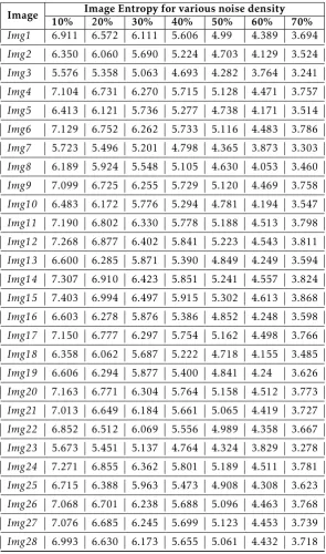
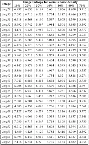
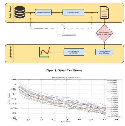
In figure 1, the over all process flow diagram of the proposed approach is shown. We have chosen set of arbitrary gray-scale images from the standard image corpus and computed their entropy values. The images are then corrupted with salt and pepper noise with varying noise densities from 10% to 70%. Each time on adding the noise, the corresponding entropy value is calculated and recorded. The variation of entropy with varying noise density for the given set of test images is shown in table1,2.
The values in table 1and 2clearly indicates that the entropy value decrease with increase in noise but there is no constant pattern for this change, only we know that entropy decrease when noise increase. In order to find the relationship between entropy and noise density, we calculated the first order difference of the entropy values of all the test images with varying noise density. We tested with 55 test images, table 3shows sample of the first order difference of entropy with respect to noise density.
The behavior of the first order entropy values and noise density is shown in figure 2. The curves clearly indicates that entropy decrease with increase in noise. Using the behavior of first order entropy values we try to find the approximate curve that will exhibit the behavior of all the curves. There are so many techniques for doing this like averaging, mean, median, most likelihood and many more.
From the statistical data obtained from the experi-ments, we use quadratic polynomial fitting according to the minimum mean square error criteria to the fitting all the first order entropy variation. Figure 3shows the graphical representations of the generalization of the relation. Equation 1 represents the intrinsic relation-ships between the noise density and the entropy value of the noise images. Here, the x denotes the second order entropy value of the noise images, f represents the noise density.
F(x) =p1x4+p2x3+p3x2+p4x+p5 (1) wherep1=−246.3
Table 1. Change in entropy with respect to noise density
Image Image Entropy for various noise density
10% 20% 30% 40% 50% 60% 70%
Img1 6.911 6.572 6.111 5.606 4.99 4.389 3.694
Img2 6.350 6.060 5.690 5.224 4.703 4.129 3.524
Img3 5.576 5.358 5.063 4.693 4.282 3.764 3.241
Img4 7.104 6.731 6.270 5.715 5.128 4.471 3.757
Img5 6.413 6.121 5.736 5.277 4.738 4.171 3.514
Img6 7.129 6.752 6.262 5.733 5.116 4.483 3.786
Img7 5.723 5.496 5.201 4.798 4.365 3.873 3.303
Img8 6.189 5.924 5.548 5.105 4.630 4.053 3.460
Img9 7.099 6.725 6.255 5.729 5.120 4.469 3.758
Img10 6.483 6.172 5.776 5.294 4.781 4.194 3.547
Img11 7.190 6.802 6.330 5.778 5.188 4.513 3.798
Img12 7.268 6.877 6.402 5.841 5.223 4.543 3.811
Img13 6.600 6.285 5.871 5.390 4.849 4.249 3.594
Img14 7.307 6.910 6.423 5.851 5.241 4.557 3.824
Img15 7.403 6.994 6.497 5.915 5.302 4.613 3.868
Img16 6.603 6.278 5.876 5.386 4.852 4.248 3.598
Img17 7.150 6.777 6.297 5.754 5.162 4.498 3.766
Img18 6.358 6.062 5.687 5.222 4.718 4.155 3.485
Img19 6.606 6.294 5.877 5.400 4.841 4.24 3.626
Img20 7.163 6.771 6.304 5.764 5.158 4.512 3.773
Img21 7.013 6.649 6.184 5.661 5.065 4.419 3.727
Img22 6.852 6.512 6.069 5.556 4.989 4.358 3.667
Img23 5.673 5.451 5.137 4.764 4.324 3.829 3.278
Img24 7.271 6.855 6.362 5.801 5.189 4.511 3.781
Img25 6.715 6.388 5.963 5.473 4.908 4.308 3.623
Img26 7.068 6.701 6.238 5.688 5.096 4.463 3.768
Img27 7.076 6.685 6.245 5.699 5.123 4.453 3.739
Img28 6.993 6.630 6.173 5.655 5.061 4.432 3.718
p3=−10.2 p4=−1.012 p5=−0.00826
The above equation indicates the relation between the first order difference entropy value and the noise density in quantitative form. This relation is extended to analyze some of the data points for calculating residuals.
4. Mathematical model formulation
The ergodic physical nature of the images can be analyzed using statistical techniques. In order to capture the degree of probability concentration and amount of randomness Hidden Markov Model transition parameters can be used. In Markov chain, there exists a positive probability measure at stage n that is independent of the probability distribution at initial stage 0. Let P be the definite random variable
3
EAI Endorsed Transactions on
Energy Web and Information Technologies
Table 2. Change in entropy with respect to noise density....Continuation
Image Image Entropy for various noise density
10% 20% 30% 40% 50% 60% 70%
Img29 6.997 6.636 6.169 5.66 5.056 4.400 3.715
Img30 7.092 6.710 6.253 5.724 5.117 4.466 3.773
Img31 6.918 6.568 6.100 5.597 5.005 4.399 3.696
Img32 5.992 5.742 5.397 4.984 4.504 3.985 3.392
Img33 4.171 4.125 3.989 3.771 3.506 3.170 2.777
Img34 5.515 5.320 5.016 4.665 4.250 3.769 3.233
Img35 6.045 5.785 5.432 5.013 4.535 3.995 3.403
Img36 6.474 6.173 5.773 5.302 4.789 4.197 3.552
Img37 6.594 6.273 5.867 5.388 4.842 4.239 3.591
Img38 5.962 5.712 5.368 4.959 4.498 3.963 3.380
Img39 5.116 4.963 4.718 4.404 4.024 3.590 3.082
Img40 6.142 5.874 5.512 5.084 4.593 4.045 3.434
Img41 5.886 5.649 5.316 4.917 4.454 3.942 3.357
Img42 5.646 5.434 5.127 4.754 4.32 3.828 3.274
Img43 7.043 6.683 6.215 5.692 5.094 4.464 3.739
Img44 6.908 6.556 6.109 5.599 5.024 4.388 3.69
Img45 7.324 6.93 6.434 5.877 5.251 4.566 3.842
Img46 3.822 3.66 3.453 3.212 2.933 2.636 2.308
Img47 7.081 6.701 6.245 5.712 5.130 4.467 3.732
Img48 4.605 4.352 4.060 3.736 3.371 2.984 2.561
Img49 7.127 6.755 6.279 5.739 5.146 4.483 3.775
Img50 4.276 4.064 3.802 3.515 3.189 2.837 2.448
Img51 7.080 6.717 6.247 5.718 5.108 4.458 3.750
Img52 6.912 6.563 6.106 5.603 5.036 4.394 3.734
Img53 4.689 4.428 4.120 3.785 3.416 3.019 2.592
Img54 6.795 6.449 6.019 5.511 4.944 4.327 3.651
Img55 7.116 6.741 6.27 5.735 5.134 4.482 3.756
Table 3. First order deviation of entropy with respect to noise density
(10 - 20)% (20-30)% (30-40)% (40-50)% (50-60)% (60-70)%
Img1 -0.3392 -0.4609 -0.5058 -0.6154 -0.6015 -0.6940
img9 -0.3732 -0.4706 -0.5262 -0.6089 -0.6510 -0.7102
with probability Mass function andP pi is the entropy given by
H(P)− L−1 X
i=0
(P pi)∗log(P pi)
Figure 1. System Flow Diagram
Figure 2. First order Entropy vs Noise Density
Figure 3. Generalization of data points
5
EAI Endorsed Transactions on
Energy Web and Information Technologies
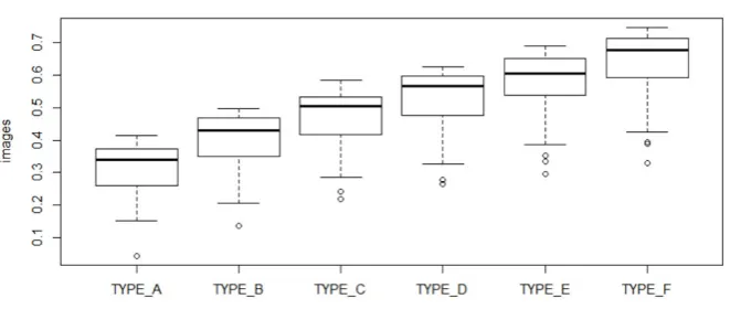
Welch test the uncertainties can be eliminated. By using statistical techniques for different images and based on the various types the values obtained are as shown in table 4. Here TYPE_A denotes the first order entropy difference between noise 10 and 20% densities of test images, TYPE_B denotes the first order entropy difference between noise 20 and 30% densities, TYPE_C denotes the first order entropy difference between noise 30 and 40% densities, TYPE_D denotes the first order entropy difference between noise 40 and 50% densities, TYPE_E denotes the first order entropy difference between noise 50 and 60% densities, TYPE_F denotes the first order entropy difference between noise 60 and 70% densities.
Using the behavior of first order entropy, the correlation coefficient has been obtained and its value is 0.9767652, the error estimated is 8.9% and this first order entropy changes has been depicted in figure4.
5. Conclusions
In this paper, the relationship between the entropy values of images and the noise for the salt & pepper noise is being analyzed. It reveals to the fact that the entropy value diminishes more and more while the density of salt and pepper noise in the noisy image becomes larger and larger, and such relation is robust to individual image traits. By using using Lagrange interpolating polynomial to describe the variation of second order entropy with noise density curve fitting is obtained. Using the behavior of first order entropy, the correlation coefficient has been obtained and its value is 0.9767652, and the error estimated is 8.9%. Hence based on the numerical calculation and graphical relation, our proposed technique and analysis can be considered as an approach with minimum residual for salt & pepper noise density estimation.
References
[1] Agarwal, T.,Jha, S.andKanna, B.R.(2013) P-HGRMS:
A parallel hypergraph based root mean square algorithm for image denoising.CoRR abs/1306.5390. URL http: //arxiv.org/abs/1306.5390.
[2] Chao Z H, Li Y J, Z.K. (2006) Estimation of salt
and pepper noise on the magnitude spectrum.Infrared Technology28(9): 549–551.
[3] Cheng-Jun, Z. (2013) Entropy-based estimation of
salt-pepper noise in wavelet domain. In Wavelet Active Media Technology and Information Processing, 10th International Computer Conference on: 366–370. doi:10.1109/ICCWAMTIP.2013.6716668.
[4] Cover, T.M. and Thomas, J.A. (1991) Elements of
Information Theory (New York, NY, USA: Wiley-Interscience).
[5] Dharmarajan, R.andKannan, K.(2010) A
hypergraph-based algorithm for image restoration from salt and pepper noise. AEU - International Journal of Electronics and Communications 64(12): 1114 – 1122. doi:http://dx.doi.org/10.1016/j.aeue.2009.12.001, URL
http://www.sciencedirect.com/science/article/
pii/S143484110900332X.
[6] Gallagher, N.C., J. andWise, G.(1981) A theoretical
analysis of the properties of median filters. Acoustics, Speech and Signal Processing, IEEE Transactions on29(6): 1136–1141. doi:10.1109/TASSP.1981.1163708.
[7] Hwang, H.andHaddad, R.(1995) Adaptive median
fil-ters: new algorithms and results.Image Processing, IEEE Transactions on4(4): 499–502. doi:10.1109/83.370679.
[8] Kannan, K., B, R.K.. and Aravindan, C. (2010) Root
mean square filter for noisy images based on hyper graph model.Image and Vision Computing28(9): 1329 – 1338. doi:http://dx.doi.org/10.1016/j.imavis.2010.01.013,
URL http://www.sciencedirect.com/science/
article/pii/S0262885610000296.
[9] Peng, Q. and Run-Tao, D. (2004) Ordering threshold
switching median filter. Journal of Image and Graphics
9(4): 412–416.
[10] Shannon, C.E. (1948) A mathematical theory of
com-munication.Bell System Technical Journal27(3): 379–423. doi:10.1002/j.1538-7305.1948.tb01338.x, URL http:// dx.doi.org/10.1002/j.1538-7305.1948.tb01338.x.
[11] SONG Yu, LI Man-Tian, S.L.N. (2007) Image salt and
pepper noise self-adaptive suppression algorithm based on similarity function.Acta Automatica Sinica33(5): 474. doi:10.1360/aas-007-0474, URLhttp://www.aas.net. cn/EN/abstract/article_14293.shtml.
[12] Wang, Z. and Zhang, D. (1998) Restoration of
impulse noise corrupted images using long-range correlation. Signal Processing Letters, IEEE 5(1): 4–7. doi:10.1109/97.654865.
[13] Wang, Z.andZhang, D.(1999) Progressive switching
median filter for the removal of impulse noise from highly corrupted images.Circuits and Systems II: Analog and Digital Signal Processing, IEEE Transactions on46(1): 78–80. doi:10.1109/82.749102.
[14] Xing Z. J, Wang S. J, D.H. (2001) A new filtering
algorithm based on extremum and median value.Journal of Image and Graphics6(6): 533–536.
[15] Xu, H.,Zhu, G.,Peng, H.andWang, D.(2004) Adaptive
fuzzy switching filter for images corrupted by impulse noise. Pattern Recognition Letters 25(15): 1657 – 1663. doi:http://dx.doi.org/10.1016/j.patrec.2004.05.025,
URL http://www.sciencedirect.com/science/
article/pii/S0167865504001151.
[16] Zhang Q, Liang D. Q, F.X.(2004) Identifying of nosie
types and estimating of noise level for a noisy image in the wavelet domain.Journal of Infrared Millimeter Waves
Table 4. Noise Density with respect to first order change in entropy
TYPE_A TYPE_B TYPE_C TYPE_D TYPE_E TYPE_F
Min. 0.04557 0.1362 0.2181 0.2655 0.2973 0.3286
1st Qu. 0.26033 0.3490 0.4165 0.4763 0.5373 0.5923
Median 0.33915 0.4297 0.5028 0.5662 0.6047 0.6766
Mean 0.31310 0.4027 0.4695 0.5275 0.5823 0.6385
3rd Qu. 0.37294 0.4677 0.5310 0.5968 0.6511 0.7121
Max. 0.41507 0.4973 0.5826 0.6255 0.6896 0.7448
Variance 0.00589 0.0068 0.0075 0.0085 0.0091 0.01009
Figure 4. Change in entropy with increased noise density
7
EAI Endorsed Transactions on
Energy Web and Information Technologies