PERFORMANCE ANALYSIS OF SELECTIVE HARMONIC ELIMINATION BASED COMPENSATION CONTROL FOR SHUNT ACTIVE POWER FILTER

PERFORMANCE ANALYSIS OF

SELECTIVE HARMONIC

ELIMINATION BASED

COMPENSATION CONTROL FOR

SHUNT ACTIVE POWER FILTER

UNNATI MODI

Student, Department of Electrical Engineering, Institute of Technology, Nirma University, Ahmedabad-382481, Gujarat, India.

[email protected]

TEJPAL TOSAR

Student, Department of Electrical Engineering, Institute of Technology, Nirma University, Ahmedabad-382481, Gujarat, India.

[email protected]

SIDDHARTHSINGH K. CHAUHAN

Associate Professor, Department of Electrical Engineering, Institute of Technology, Nirma University, Ahmedabad-382481, Gujarat, India.

[email protected]

Abstract:

Due to wide use of nonlinear loads, source current gets distorted. Shunt APF is used to mitigate the harmonics from source current and reduce the THD in source current. Reference currents are generated using Selective Harmonics Elimination method. These reference currents are injected to the point of common coupling to eliminate the dominant harmonics present in the source current. The steady state experimental waveforms show that good filtering characteristic is achieved. Also the FFT analysis of source and load currents show that the dominant harmonics present in load current are eliminated from source current waveform. Multilevel inverters are recently used for active filter topologies. They have many advantages such as lower harmonic distortion, lower switching frequency and reduced switching losses over two-level Inverters. In this paper, performance analysis of two-level and three-level Inverter based APF is presented. To verify the performance, MATLAB simulated results are described here.

Key words: APF (Active power filter), SHE (Selective Harmonics Elimination), Harmonics, THD 1. INTRODUCTION

Nowadays, harmonic current flowing into grid is growing due to the presence of nonlinear loads in the system. Nonlinear loads draw non-sinusoidal currents from supply and cause reactive power burden and inject harmonics. This harmonic-distortion current has to be minimized to mitigate power quality issues. To provide high power quality at the point of common coupling (PCC) of a system, active power filters (APF) are widely used. Active filters provide dynamic and adjustable solution of the power quality problems. It is also called active power line conditioners. It can compensate current and voltage harmonics, reactive power, regulate terminal voltage and improve voltage balance in three phase system. The advantages of active power filters are: 1) Automatically adapts to change in networks and load fluctuations

There are three types of APF named Shunt APF, Series APF and Hybrid APF. Among these we have used Shunt APF for load current harmonics compensation. Shunt APF is the most widely used type in active filter application. The purpose is to mitigate the load current harmonics fed to the supply [1].

Fig.1 Shunt APF

Shunt APF generates current having magnitude same as harmonics present in the load current and 180° phase shifted from it. It will inject it to the point of common coupling (PCC) and due to it, THD in the source current will decrease. For generation of proper compensating current, proper reference current must be generated. There are different techniques for reference current generation in time domain like instantaneous reactive power theory, synchronous reference frame theory, selective harmonics elimination etc. Also FFT technique is used to generate reference current in frequency domain. Among these, Selective Harmonics Elimination (SHE) technique for reference current generation is used here.

2. SHE PRINCIPLE

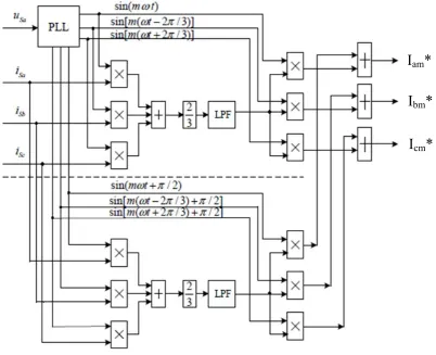
This technique has been introduced to reduce the dominant harmonics which are chosen by the designer. It requires only knowledge of the frequency of the harmonic component to be eliminated. The main idea behind this technique is to generate a reference current by the usual method and, then, to process their harmonics individually. A new reference current is then produced with information about the most problematic harmonics that need to be eliminated. Reduced filter rating and reduced current-control bandwidth are the main advantages of this technique. This technique can be applied to single phase as well as three phase APF applications. As shown in Fig.2 [2], the value of frequency and phase angle of three phase source voltage USa can be obtained

by passing it through PLL. Using the value of ωt, m and iSa, iSb andiSc, the value of Iq and Id are acquired from

following equations. Here, m= order of harmonic to be eliminated. Iam*, Ibm* and Icm* are reference current for

three phases.

Iq 2₃ – ila*sin mωt – ilb* sin m ωt-2π₃ – ilc*sin m ωt 2π₃ (1)

Fig. 2 Diagram to generate the m-order harmonic current

Then these Iq and Id are passed through first order LPF. Then from these values of Id* and Iq*, three phase

reference currents iam*, ibm* and icm* for mth order of harmonic is obtained by using following equations

∗ ∗_{sin ω} ∗ _{cos(mωt) (3)}

∗ ∗_{sin ω} ∗_{cos ω (4)}

∗ ∗_{sin ω} ∗_{cos ω (5)}

3. HYSTERESIS CURRENT CONTROLLER

Selection of controller significantly affects the performance of Shunt APF because Current controllers force the actual compensating current supplied by APF at PCC to track the reference compensating current generated by mathematical computations. There are different types of current controllers which are used in shunt APFs, among which hysteresis controllers are widely used because of their inherent simplicity and fast dynamic response. Hysteresis controllers make the actual compensating current to be within the hysteresis band by the switching action of the SAPF.

Iam*

Ibm*

3.1 Switching signal generation for two level SAPF

Fig. 3 Two-level hysteresis current control

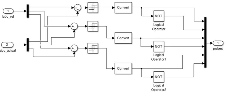
Fig. 4 Logic to generate switching pulses for SAPF

In hysteresis current control, we set the upper band and lower band for actual current. This band will act as limit within which controller will make actual current to track the reference current. Relay is used for this purpose. Difference of reference current and actual current passes through the relay. When actual current hits the upper band, voltage should be decreased. So relay will be turned off and lower switch of the leg will get gate pulse and –Vdc will appear across that leg. Similarly when actual current hits the lower band, voltage should be increased.

So relay will be turned on and upper switch of the leg will get gate pulse and +Vdc will appear across that leg.

The on/off state of the relay is not affected by input between upper and lower limit.

3.2 Switching signal generation for three level SAPF

Fig. 5 Three-level hysteresis current control

Fig. 6 Logic to generate switching pulses for SAPF

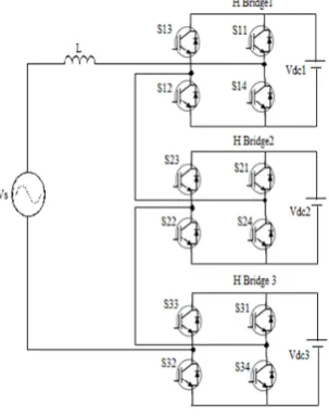
Here, H-Bridge topology of three phase three-level Inverter is used. Schematic diagram of three-level Inverter is shown in Fig. 7.

• Switching algorithm for three-level inverter [3]

For e > 0: positive half cycle

1. Switch S11 remains ON and the complimentary switch S14 remains OFF.

2. If e > (h+δ) then S12 is ON and S13 is OFF.

3. If e < δ, then S13 is ON and S12 is OFF.

For e < 0: Negative half cycle

1. Switch S14 remains ON and the complimentary switch S11 remains OFF.

2. If e < -(h+δ) then S13 is ON and S12 is OFF.

3. If e > -δ, then S12 is ON and S13 is OFF.

Here, e = error which shows the difference of actual current and reference current

h = hysteresis limit which act as a limiter within which controller will make actual current to track the reference current.

δ = 0.01, which is dead band zone.

4. SIMULATION RESULTS

To verify the proposed SHE scheme, simulation studies are performed in MATLAB simulation software for two-level as well as three-level Inverter based APF. This simulation is done for 0.08 sec which contain four cycles.

4.1Two level Inverter based APF

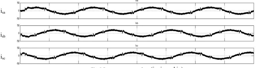
Fig. 8 shows the three phase source current (isa, isb and isc) waveforms.

Fig. 8 Source current waveform (isa, isb and isc)

Fig. 9 shows the three phase load current (ila, ilb and ilc) waveforms.

Fig. 9 Load current waveform (ila, ilb and ilc)

These current waveforms are observed for two-level Inverter based APF while keeping coupling Inductor as 100uH and hysteresis band value as 3.00. Coupling Inductor is used for the smoothening of the current waveform and is connected between point of common coupling (PCC) and Inverter. As shown in Fig. 8 and Fig.

Fig. 10 shows the tracking of actual current and reference current. X-axis represents time (sec) and Y-axis represents current (A). Here, waveform in black colour shows actual current waveform and pink colour waveform shows reference current waveform. It is observed from above figure that reference current is tracking properly which means Hysteresis Current Controllers are working properly.

Fig. 10 Actual current and reference current waveform

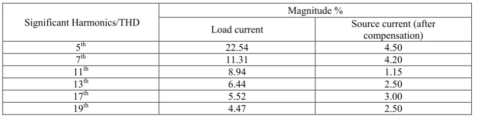
As shown in table 1, Harmonic content is reduced in source side after compensation. THD is observed 28.47% before compensation and 8.05 % after compensation. Fig. 11 shows FFT plot of the load current before compensation and Fig. 12 shows FFT plot of the source current after compensation. In both figures, X-axis indicates Harmonic order and Y-axis indicates Fundamental magnitude in %.

Table 1 Comparison of Harmonic component present in Load current and Source current after compensation.

Significant Harmonics/THD _{Load current} Magnitude % Source current (after compensation)

5th _{22.54 4.50}

7th _{11.31 4.20}

11th _{8.94 1.15}

13th _{6.44 2.50}

17th _{5.52 3.00}

Fig. 11 FFT plot of load current before compensation Fig. 12 FFT plot of source current after compensation

From the above FFT plots, it is observed that harmonic content is being reduced after compensation.

4.2Three level Inverter based APF

As shown in Fig. 7, three-level H-bridge Inverter is used here. DC link voltage is kept as 700 V in simulation to check the performance of three-level Inverter based APF.

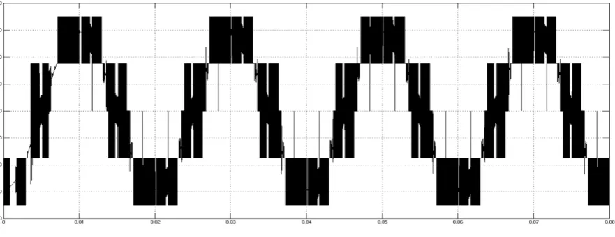
Fig. 13 shows the line voltage waveform. Since Hysteresis current controller is employed here, some randomness in Line voltage waveform is observed. Otherwise Fig. 13 shows the expected waveform of Line voltage. X-axis represents time (sec) and Y-axis represents voltage (V).

Fig. 13 Line voltage waveform

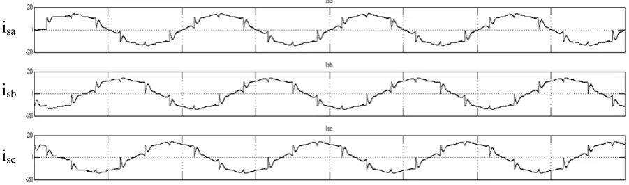
Fig. 14 and Fig. 15 show simulated results of three phase source current (isa, isb and isc) and;load current (ila, ilb

Fig. 14 Source current waveform (isa, isb and isc)

Fig. 15 Load current waveform (ila, ilb and ilc)

Fig. 16 Actual current and reference current waveform

Fig. 16 shows the tracking of actual current and reference current. X-axis represents time (sec) and Y-axis represents current (A). Here, waveform in black colour shows actual current waveform and pink colour waveform shows reference current waveform. It is observed from above figure that reference current has expected shape (M-W) but there is some mismatch in tracking which is due to Hysteresis controller.

i

i

i

i

i

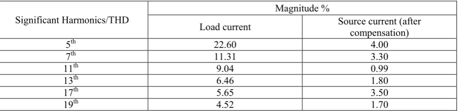
Table 2 Comparison of Harmonic component present in Load current and Source current after compensation.

Significant Harmonics/THD Magnitude %

Load current Source current (after _{compensation)}

5th _{22.60 4.00}

7th _{11.31 3.30}

11th _{9.04 0.99}

13th _{6.46 1.80}

17th _{5.65 3.50}

19th _{4.52 1.70}

As shown in table 2, Harmonic content is reduced in source side after compensation. THD is observed 28.55% before compensation and 6.87 % after compensation. Fig. 17 shows the FFT plot of the load current before compensation and Fig. 18 shows the FFT plot of the source current after compensation. In both figures, X-axis indicates Harmonic order and Y-axis indicates Fundamental magnitude in %.

Fig. 17 FFT plot of load current before compensation Fig. 18 FFT plot of source current after compensation

Fig. 17 and Fig. 18 show that harmonic content is reduced after compensation. It is clearly observed from above FFT plots.

Table 3 Comparison of THD

S. no. Inverter type Before compensation (%) After compensation (%)

1 Two-level Inverter based APF 28.47 8.05

2 Three-level Inverter based APF 28.55 6.87

Table 3 shows the comparison of THD (%) for two-level and three-level Inverter based APF. It is observed that three-level Inverter based APF is more effective than two-level Inverter based APF.

5. CONCLUSION

References

[1] M.EI-Habrouk, M.K.Darwish and P.Mehta, “Active power filters: A review”

[2] Chen Junling, Li Yaohua, Wang Ping, Yin Zhizhu and Dong Zuyi, “A Closed-Loop Selective Harmonic Compensation with Capacitor

Voltage Balancing Control of Cascaded Multilevel Inverter for High power Active Power Filters”

[3] Shweta Gautam and Rajesh Gupta, “Switching Frequency Derivation for the Cascaded Multilevel Inverter Operating in Current