THERMAL MODELING OF
AIR-CONDITIONED PROTOTYPE ROOM
USING MATLAB-SIMULINK
C. B. PATIL
Department of Electronics, D. K. A. S. C. College, Ichalkaranji, Maharashtra, INDIA-416115 Telephone: +919922049750, Email- [email protected]
S. R. POTDAR
Department of Physics; Arts, Science and Commerce College, Rahata, Maharashtra, INDIA-423107 Email- [email protected]
R. R. MUDHOLKAR
Department of Electronics, Shivaji University, Kolhapur, Maharashtra, INDIA-416004 Email- [email protected]
Abstract: The paper reports the design and development of simplified thermal model of a prototype room and air-conditioner in Matlab-Simulink environment. For establishment of model, the physical properties of room and air-conditioner have taken into account. The heat transfer among the prototype room has modeled using energy conservation equations. While the vapor compression based air conditioner has modeled using transfer function which is derived experimentally. The total system model so developed has simulated for different compressor speeds, different outside temperatures as well as for different wall materials. The results obtained offer the information pertaining to heat extraction by the air conditioner as well as heat gain through the walls. It also explores the temperature variation within the room for different scenarios. Thus the designed model is helpful in estimating the size of an air-conditioner. It further helps to design a control system as well. The developed model has verified experimentally. It is observed that simulated result and experimental result are in good agreement.
Keywords: thermal modeling, air-conditioner, energy conservation equations, transfer function, Matlab-Simulink
1. Introduction
Now in global warming era, it is requisite to work on reduction and optimization of the energy consumption in various fields, one such field is the residential sector. In residential sector the main energy consuming device is the HVAC (Heating, Ventilation and Air Conditioning) systems used for heating or cooling buildings. So to optimize the energy consumption in HVAC or Air-conditioning systems, the researchers has to be more concentrate on some important aspects as: the use of an adequate mathematical model of the building and efficient techniques to control physical parameters [Patil C. B. et al ,(2016); Radu Balan,(2011)]. To do such work the thermal performances of various elements in the whole system has to study. The thermal performance of a building refers to the process of modeling the energy transfer between a building and its surroundings. Now-a-days computer modeling is one of the widespread ways, used in the green building industry to predict energy consumption, thermal comfort and to size HVAC equipment [Roberto Padovani et al,(2011); Karmacharya et al, (2012)].
Generally the modeling can be performed in three different ways. The first category is based on physical and basic principle modeling (white-box). The second is the statistical models (black-box). Finally, the third category is a hybrid method (grey-box), which uses both physical and statistical modeling techniques [Fatima Amara et al, (2015)].
2. Mathematical Modeling of a System:
A prototype room of dimension 0.9 m long by 0.6 m wide and 1.22 m high with the total volume of 0.7 m3 made
from thermocol with thickness 0.038 m is considered for this study. A direct expansion (vapor compression) based small air conditioner is placed within that room. The air conditioner system is composed of condenser coil, vane rotary compressor with three-phase induction motor, evaporator coil and expansion devices. The prototype room is modeled using energy conservation equations as follows.
dQ
dT 1 dQextracted gain
= ( )
dt M C dt dt
room
roomair air
− (1)
Where,
Troom = room temperature = (0C)
Mroomair = mass of air inside the room = 0.83 kg
Cair = specific heat of air = 1005.4 J/kg.0C
Qextracted = heat energy extracted from the room by air conditioner = (J)
Qgain = heat energy entered inside the room through the wall by conduction = (J)
The rate of thermal energy gain through the walls is modeled using Fourier’s law of conduction as given in Eq. (2),
dQ
room - outside
= ( ) dt R T T gain (2) Where,
Toutside = outside temperature
R = Thermal resistance of wall
= ( t ) R
kA (3)
Where,
t = thickness of wall = 0.038 m
k = thermal conductivity value of thermocol of density (ρ = 0.05 g/cm3) = 0.033 W/m0C
A = Area of wall = 4.8 m2
Since the evaporator is placed inside the room, the refrigerant through it absorbs the heat from the room. Thus the rate of thermal energy extracted (Qextracted) by the Air-conditioner from the room is modeled by using mass
flow rate of air as in Eq. (4),
dQ dM
= ( Tac Troom)
dt dt
extracted air C
air − (4)
Where,
dMair/dt = mass flow rate of air = ρ. v. Ac (5)
Where ρ = density of air = P/RT (6)
Where P = Absolute pressure = 100 kPa
R = Gas constant = 0.287 kPa.m3/kg.K
T = Absolute temperature = (33+273) = 306 K Thus, ρ = 1.14 kg/m3
v = air flow velocity = 0.35 m/s
Ac = cross-sectional area of blower duct = 0.034 m2
dMair/dt = 0.014 kg/s
Tac = evaporator_coil_temperature = (0C)
Since mass flow rate of air is kept constant, then dQ
= M ( Tac Troom) dt
extracted C
air air − (7)
Since evaporator_coil_temperature (Tac) is a varying quantity and is dependent on speed of compressor,
surrounding temperature and mass flow rate of air. So to model Tac , a step response experiment has been carried
out. A step signal of 5.75 V has been applied to the input of Air- conditioner system which drives the compressor to run at 1600 rpm and then the corresponding evaporator_coil_temperature has been logged. The data thus obtained is plotted as shown in figure 1.
Fig: 1 Evaporator_coil_Temperature
Then to derive the transfer function of vapor compression based small air conditioner system, a system of first order has been considered. So the first order transfer function will be of the form
( ) = 1 K G s
Ts+ (8)
The term G(s) denotes the Laplace transform, of the gain of the system between the change in the control voltage (meaning change in compressor speed) and the change in the system temperature. Here K is the gain and T is time constant of a system. Let the change in the control voltage be denoted by u and change in temperature be denoted by y. Then we obtain the following relation between the control voltage and temperature.
( ) = G ( ). u( )
y s s s (9)
( ) = . 1
K u
y s
Ts s
Δ
+ (10)
Since we are applying step input, Δu is constant. By applying Inverse Laplace transform we get,
( / ) ( ) = K[1- e t T ].
y s − Δu (11)
From Eq. (11), it is seen that the temperature Tac varies inversely.
Here, K = change in temperature / change in input step signal = (33-12)/ 5.75 = 3.65
T = time constant = 70 s (from graph)
Substituting the above values, the Transfer function will be, 3.65
( ) = 70 1 G s
s+
(12)
By considering above Transfer function, the Evaporator_coil_temperature (Tac) has been modeled in
MATLAB_SIMULINK as shown in figure 2
Also a Transfer function is converted into a first order differential equation as given in Eq. (13).
3.65
- = ( )
70 70
dy y
u s
dt (13)
Again by considering differential Eq. (13), the Evaporator_coil_temperature has been modeled in MATLAB_SIMULINK as shown in figure 3
Fig: 3 SIMULINK model to obtain Evaporator_coil_temperature using Differential equation
Simulated results of both the models have been plotted as shown in figure 1 and are in good agreement to the experimental result.
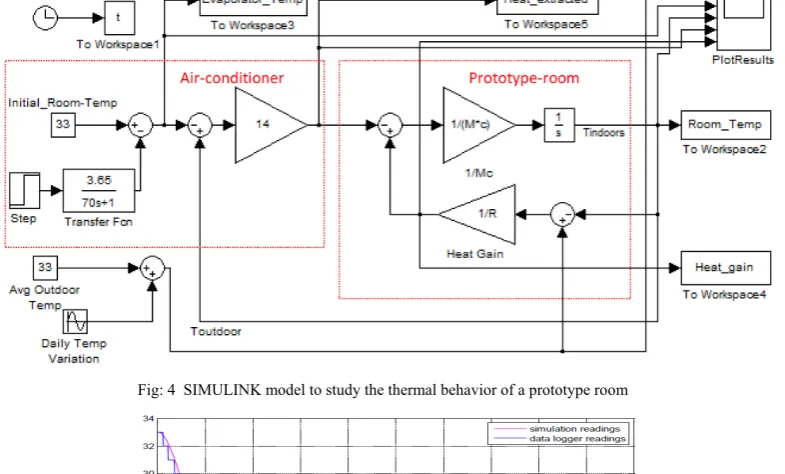
Further a room air temperature is being modeled in MATLAB_SIMULINK using above thermal model of air-conditioner and energy conservation equations as shown in figure 4. The simulated result plotted is as shown in figure 5.
Fig: 4 SIMULINK model to study the thermal behavior of a prototype room
Fig: 5 Room_air_Temperature
3 Experimental studies:
In order to verify the simulated result, an experiment has been carried out by providing the same step signal of 5.75 V to the input of Air- conditioner system. Then the corresponding room_air_temperature has been logged. The data thus obtained is plotted as shown in figure 5. It is observed that simulated result and experimental result are in good agreement.
Fig: 6 Variation in Evaporator_coil_temp, Room_air_Temperature, Heat extracted by Air-conditioner and Heat gain through walls
Fig: 7 Variation in Evaporator_coil_temp for different compressor speeds
Fig: 9 Variation in Room_air_temp for different wall materials
Fig: 10 Variation in Heat-gain for different wall materials
4 Result and Analysis:
From figure 6, it is observed that in transition state, heat energy extracted by the Air-conditioner and heat energy gain from walls has drastic change. It is observed that the maximum heat energy extraction reached to about 105 joules/sec and then after it remains constant around 58 joules/sec. Similarly heat gain also reached to around 58 joules/sec at steady state. When heat energy extracted and gained becomes equal, the system goes into steady state. So the room_air_temperature remains to its steady state value around 15 0C.
The Simulink model has been evaluated for different control voltages meaning different compressor speeds. The results plotted in figure 7, shows that Tac and Ta values decreases with increasing compressor speed,
meaning that rate of heat extraction has increased. Thus the room gets colder with increase in compressor speed. The model has been simulated for different outside temperature. The variations in room_air_temperature are shown in figure 8. It is observed that increase in outside temperature, increases the values of both Tac and Ta, meaning that rate of heat gain has increased. Thus the room gets hotter with increase
in outside temperature.
Also the model has been simulated for different room materials such as common red burnt brick (k value = 0.8 W/m0C ) having thickness of 0.227 m (9” inch) with 0.0254 m (1” inch) plaster (k value = 0.7
W/m0C) and another with same brick with 0.05 m (2” inch) styrofoam (k value = 0.033 W/m0C) and 0.013 m
(0.5” inch) fiber board (k value = 0.048 W/m0C). The simulated result in figure 9 shows that for good insulated
room, the room_air_temperature is far below about 8 0C than un-insulated room. From figure 10, it is seen that
the thermal gain was reduced from 150 joules/sec to 45 joules/sec, when room is transformed into well insulated room.
5 Conclusion:
Thermal modeling of a prototype building offers information pertaining to the heat extraction by the air conditioner as well as heat gain through the walls for different scenarios. So it is helpful in estimating the size of an air-conditioner. It further helps to design a control system as well. The thermal insulations in roof and walls reduce the heat gain, which reduces the operating time of an air-conditioner thereby reducing the annual energy cost for a building.
References
[1] Patil C. B. et al,(2016):Thermal Modeling and Fuzzy Logic Temperature Controller for Prototypical Room, International Journal of
Engineering Trends and Technology (IJETT) – Volume 36 Number 8 – June 2016,
[2] Radu Balan,(2011):Thermal modelling and temperature control of a house, The Romanian Review Precision Mechanics, Optics &
Mechatronics, , No. 39
[3] Roberto Padovani et al, (2011): Dynamic Thermal Modelling and CFD Simulation Techniques used to innluence the design process in
Buildings, Proceedings of Building Simulation 2011:12th Conference of International Building Performance Simulation Association, Sydney, 14-16 November.
[4] Karmacharya et al, (2012):Thermal modelling of the building and its HVAC system using Matlab/ Simulink, EFEA 2012: 2nd
International Symposium on Environment Friendly Energies and Applications, 25-27 July 2012, Northumbria University, Newcastle upon Tyne, UK.
[5] Fatima Amara et al,(2015): Comparison and Simulation of Building Thermal Models for Effective Energy Management, Smart Grid