Autoregressive Models
INAUGURAL-DISSERTATION
zur Erlangung des akademischen Grades eines Doktors der Wirtschaftswissenschaft
doctor rerum politicarum
(Dr. rer. pol.)
am Fachbereich Wirtschaftswissenschaft der Freien Universität Berlin
vorgelegt von Annika Schnücker
Zweitgutachter: Prof. Dr. Dieter Nautz
Professur für Ökonometrie Freie Universität Berlin
First and foremost, I am grateful for the support, advice, and encouragement of my su-pervisor Helmut Lütkepohl. He gave me the opportunity to work independently on my preferred topics and provided constant guidance. I would also like to thank my second supervisor, Dieter Nautz, for his support and comments. I am very thankful to Tomasz Woźniak for giving me the opportunity to visit the University of Melbourne, for being an extremely attentive and kind host, and for fruitful discussions. I thank my co-author Gregor von Schweinitz for the productive and inspiring cooperation. I am also grateful for the constructive questions and comments of the participants of the regular Seminar Empirical Macroeconomics of the Freie Universität Berlin.
I wrote this dissertation as a member of the DIW Berlin Graduate Center. I am grateful for the support of the GC and the great environment. In particular, I thank the GC macro PhD students for hours of discussions and my GC 2013 cohort for a memorable first year. I thank the GC team and especially Juliane Metzner and Georg Weizsäcker for their support and understanding particularly during the job market.
I am grateful to my officemates and friends, Niels Aka and Hedwig Plamper, for enjoy-able conversations beyond economics and GC work. I also thank Pablo Anaya Longaric, Daniel Bierbaumer, Caterina Forti Grazzini, Marie Le Mouel, and Ulrich Schneider for uncountable lunches, coffee breaks, and their friendship outside the DIW.
I thank my family for their encouragement, their belief in me, and for fully endorsing my decisions and priorities. Above all, I am extremely grateful for the endless support and patience of Georg.
Berlin, May 2018 Annika Schnücker
Diese Dissertation besteht aus drei (Arbeits-)Papieren, von denen eines in Zusammen-arbeit mit einem Koautor entstanden ist. Der Eigenanteil an Konzeption, Durchführung und Berichtsabfassung der Kapitel lässt sich folgendermaßen zusammenfassen:
• Annika Schnücker:
“Restrictions Search for Panel Vector Autoregressive Models”
Eigenanteil: 100 Prozent
• Annika Schnücker:
“Penalized Estimation of Panel Vector Autoregressive Models: A Lasso Approach”
Eigenanteil: 100 Prozent
• Annika Schnücker und Gregor von Schweinitz:
“International Monetary Policy Transmission”
Working Papers
Schnücker, A., 2016. Restrictions Search for Panel VARs. DIW Discussion Papers 1612, Berlin
Acknowledgments IV
Erklärung zu Ko-Autorenschaften V
Liste der Vorpublikationen VI
List of Figures XI
List of Tables XIII
List of Abbreviations XV
Summary XVII
Zusammenfassung XIX
Introduction and Overview XXI
1 Restrictions Search for Panel Vector Autoregressive Models 1
1.1 Introduction . . . 1
1.2 Literature . . . 3
1.3 PVAR Model Restrictions . . . 7
1.4 Selection Prior for PVAR Models . . . 8
1.5 Monte Carlo Simulation . . . 12
1.5.1 Simulation Set-Ups . . . 12
1.5.2 Results . . . 14
1.6 Empirical Application . . . 18
1.6.1 Data and Procedure . . . 18
1.6.2 Results . . . 19
1.7 Conclusions . . . 24
1.A Gibbs Sampler Algorithm . . . 26
1.C Monte Carlo Simulation . . . 29
2 Penalized Estimation of Panel Vector Autoregressive Models 31 2.1 Introduction . . . 31
2.2 Literature . . . 34
2.3 The lasso for PVAR Models . . . 37
2.3.1 PVAR Model . . . 37
2.3.2 The lasso Estimator . . . 38
2.3.3 Extended Penalty Term and Loss Function for PVAR Models . 38 2.3.4 Asymptotic Properties . . . 43
2.3.5 Comparison to Other Estimation Procedures for PVAR Models 44 2.4 Simulation Studies . . . 47
2.4.1 Simulation Set-Ups . . . 47
2.4.2 Performance Criteria . . . 50
2.4.3 Simulation Results . . . 51
2.5 Forecasting with Multi-Country Models . . . 55
2.5.1 Forecasting Including a Global Dimension . . . 55
2.5.2 Forecasting Applications . . . 55
2.5.3 Results of the Forecasting Exercises . . . 57
2.6 Conclusions . . . 60
2.A The lasso Estimator . . . 62
2.B Estimation of the Covariance Matrix . . . 63
2.C Optimization Algorithm . . . 64
2.D Proof of Selection Consistency and Asymptotic Normality . . . 65
2.D.1 Proof of Asymptotic Normality . . . 66
2.D.2 Proof of Selection Consistency . . . 67
2.E Simulation . . . 68
2.E.1 Additional Simulation Results . . . 68
2.E.2 Simulation Results for the Model with Covariance Estimated with OLS . . . 71
2.F Forecasting Application . . . 73
2.F.1 Penalty Parameters . . . 73
2.F.2 Additional Results of the Forecasting Exercises . . . 73
3 International Monetary Policy Transmission 79 3.1 Introduction . . . 79
3.3 Cross-Border Transmission of Monetary Policy . . . 85
3.3.1 Monetary Policy in the United States, United Kingdom, and the Euro Area . . . 85
3.3.2 Transmission Channels . . . 86
3.4 Methodology . . . 88
3.4.1 Three-Country Structural VAR Model . . . 88
3.4.2 Identification of Monetary Policy Shocks . . . 90
3.4.3 Bayesian Proxy Three-Country Structural VAR Model . . . 91
3.4.4 Prior and Posterior Distributions . . . 95
3.5 Data . . . 98
3.5.1 Proxy Series . . . 98
3.5.2 Variables in the VAR Model . . . 102
3.6 Results . . . 105
3.6.1 Domestic Monetary Policy Transmission . . . 105
3.6.2 International Monetary Policy Transmission . . . 109
3.6.3 Discussion of the Results . . . 113
3.7 Conclusions . . . 116
3.A Posterior Distributions . . . 118
3.B Estimation Algorithm . . . 118
3.C Data . . . 120
3.D Prior Choices . . . 122
3.E Relevance of the Proxies . . . 123
3.F Additional Proxy VAR Results . . . 125
3.F.1 Results with High Relevance Prior for US and UK without Ad-ditional Sign Restriction on Credit Spread Variable . . . 125
3.F.2 Results with Inverse Gamma Prior . . . 128
3.F.3 Results for the EA with Different Monetary Policy Indicator . . 131
3.F.4 Results for the UK with Different Proxies . . . 131
3.F.5 Results for Three-Country VAR Models with Identified US Mon-etary Policy Shock . . . 134
Bibliography XXVII
Eidesstattliche Erklärung XXXVI
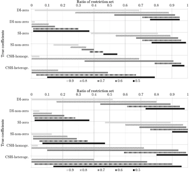
1.1 Range of posterior probabilities αlk
ij = 0, ψlkij = 0, and αlkjj = αlkii and
ratio of restriction set with threshold value 0.5 . . . 15
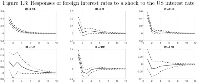
1.2 Responses of US variables to a shock to the US interest rate . . . 23
1.3 Responses of foreign interest rates to a shock to the US interest rate . 24 1.4 Share of restrictions set according to threshold value - simulations 1 and 2 29 2.1 Sparsity pattern of the coefficient matrix for model (1) . . . 59
2.2 Boxplots of MSEs and MSFEs relative to OLS for simulation 1 . . . . 69
2.3 Boxplots of MSEs and MSFEs relative to OLS for simulation 2 . . . . 70
2.4 Sparsity pattern of the coefficient matrix for model (1): lag 4 and 5 . . 77
2.5 Sparsity pattern of the covariance matrix for model (1) . . . 77
3.1 International monetary policy transmission . . . 87
3.2 Monetary policy surprise series . . . 99
3.3 Cross-correlations of monetary policy surprise series . . . 101
3.4 Model (1): Responses of US variables to a contractionary US monetary policy shock . . . 105
3.5 Model (2): Responses of UK variables to a contractionary UK monetary policy shock . . . 107
3.6 Model (3): Responses of EA variables to a contractionary EA monetary policy shock . . . 108
3.7 Model (4): Responses of exchange rates and US variables to a contrac-tionary US monetary policy shock . . . 109
3.8 Model (5): Responses of exchange rates and UK variables to a contrac-tionary UK monetary policy shock . . . 110
3.9 Model (6): Responses of exchange rates and EA variables to a contrac-tionary EA monetary policy shock . . . 111
3.10 Model (7): Responses of US, UK, and EA variables to a contractionary US monetary policy shock . . . 112
3.11 Model (8): Responses of US, UK, and EA variables to a contractionary UK monetary policy shock . . . 113 3.12 Model (9): Responses of US, UK, and EA variables to a contractionary
EA monetary policy shock . . . 114 3.13 Model (1): Posterior distributions of bU S with different priors for σv,U S 123
3.14 Model (2): Posterior distributions of bU K with different priors for σv,U K 124
3.15 Model (3): Posterior distributions of bEA with different priors for σv,EA 125
3.16 Responses of US variables to a contractionary US monetary policy shock without sign restriction . . . 126 3.17 Responses of UK variables to a contractionary UK monetary policy
shock without sign restriction . . . 127 3.18 Responses of US variables to a contractionary US monetary policy shock
- inverse Gamma prior . . . 128 3.19 Responses of UK variables to a contractionary UK monetary policy
shock - inverse Gamma prior . . . 129 3.20 Responses of EA variables to a contractionary EA monetary policy
shock - inverse Gamma prior . . . 130 3.21 Responses of EA variables to a contractionary EA monetary policy
shock - EA government bond 2-year rate as policy indicator . . . 131 3.22 Responses of UK variables to a contractionary UK monetary policy
shock - proxy of Rogers et al. (2017) . . . 132 3.23 Responses of UK variables to a contractionary UK monetary policy
shock - proxy around rate announcements of Gerko and Rey (2017) . . 133 3.24 Responses of foreign stock prices, exchange rates and US variables to a
contractionary US monetary policy shock . . . 134 3.25 Responses of foreign interest rates, exchange rates and US variables to
1.1 Deviation for estimated coefficient matrix A and Σfrom the true values 14 1.2 Accuracy of selecting DI restrictions: posterior probabilities p(αlkij = 0) 16 1.3 Accuracy of selecting SI restrictions: posterior probabilities p(ψijlk= 0) 16 1.4 Accuracy of selecting CSH restrictions: posterior probabilities p(αlk
jj =
αlk
ii) . . . 17
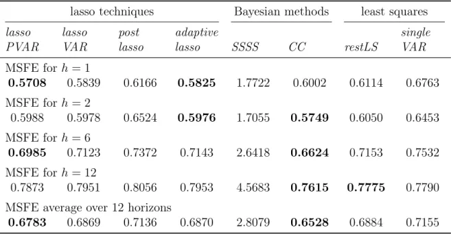
1.5 Mean squared forecast errors relative to unrestricted VAR model . . . 20
1.6 Posterior predictive density relative to unrestricted VAR model . . . . 21
1.7 10 highest posterior probabilities for the restrictions . . . 22
1.8 10 lowest posterior probabilities for the restrictions . . . 23
1.9 Hyperparameters . . . 28
2.1 Summary of simulation set-ups . . . 49
2.2 Overview of estimators . . . 51
2.3 Performance evaluation of estimators . . . 52
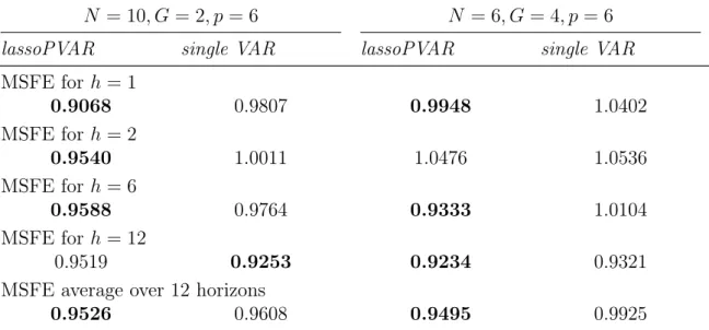
2.4 Mean squared forecast errors relative to OLS . . . 54
2.5 Overview of empirical applications . . . 56
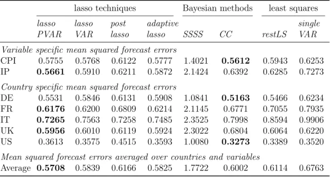
2.6 Mean squared forecast error relative to OLS for model (1) . . . 57
2.7 One-step ahead mean squared forecast error relative to OLS for model (1) . . . 58
2.8 Mean squared forecast error relative to mean forecast for model (2) and model (3) . . . 59
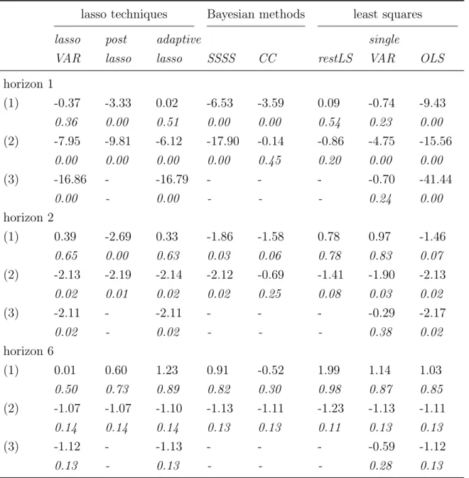
2.9 Diebold-Mariano Test: test statistic and p-values . . . 68
2.10 Performance evaluation of estimators: covariance estimated with OLS 71 2.11 Mean squared forecast errors relative to OLS: covariance estimated with OLS . . . 72
2.12 Grid values for penalty parameters - Application . . . 73 2.13 Model (1): Two-steps ahead mean squared forecast error relative to OLS 74 2.14 Model (1): Six-steps ahead mean squared forecast error relative to OLS 74
2.15 Model (1): Twelve-steps ahead mean squared forecast error relative to OLS . . . 75 2.16 Model (1): Average mean squared forecast error relative to OLS over
all forecast horizons . . . 75 2.17 Diebold-Mariano test for model (1): Test statistic and p-values - relative
to lassoPVAR . . . 76 2.18 Diebold-Mariano test for model (2) and model (3): Test statistic and
p-values - relative to lassoPVAR . . . 76 3.1 Model specifications: Individual country VAR models . . . 102 3.2 Model specifications: Three-country VAR models . . . 103 3.3 Relevance measure based on posteriors forbi and σv,i with different priors115
3.4 Variables of the United States . . . 120 3.5 Variables of the United Kingdom . . . 121 3.6 Variables of the euro area . . . 122
APD absolute percentage deviation
BMA Bayesian model averaging
BoE Bank of England
BVAR Bayesian vector autoregressive
CA Canada
CC cross-sectional shrinkage approach
CPI consumer price index
CSH cross-sectional heterogeneities
DE Germany
DGP data generating process
DI dynamic interdependencies
DK Denmark
EA euro area
ECB European Central Bank
EBP excess bond premium
EME emerging markets economies
ES Spain
FAVAR factor augmented vector autoregressive
Fed Federal Reserve System
FOMC Federal Open Market Committee
FR France
GDP gross domestic product
glasso graphical least absolute shrinkage and selection operator
GLS generalized least squares
GR Greece
GVAR global vector autoregressive
IE Ireland
IMF International Monetary Fund
IR interest rate
IT Italy
JP Japan
lasso least absolute shrinkage and selection operator
lassoPVAR least absolute shrinkage and selection operator for panel vector autoregressive models
LS least squares
MC Monte Carlo
MCMC Markov Chain Monte Carlo
MSE mean squared error
MSFE mean squared forecast error
OECD Organisation for Economic Co-Operation and Development
OLS ordinary least squares
PL predictive density
PT Portugal
PVAR panel vector autoregressive
REER real effective exchange rate
SA seasonally adjusted
SI static interdependencies
S4 stochastic search specification selection
SSSS stochastic search specification selection
SSVS stochastic search variable selection
SSVSP stochastic search variable selection for panel vector autore-gressive models
SUR seemingly unrelated regression
SVAR structural vector autoregressive
UK United Kingdom
UN unemployment rate
US United States
Multi-country dynamic time series models, called panel vector autoregressive (PVAR) models, allow for multilateral cross-border linkages and country-specific dependencies among variables. Thus, these models are excellent tools for macroeconomic spillover analyses. However, as they jointly model multiple variables of several countries, the dimensionality of unrestricted PVAR models is large and the estimation feasibility is thus not guaranteed with standard methods. Hence, model selection techniques which restrict PVAR models and thereby reduce the dimensionality of the models are necessary to ensure the estimation feasibility. Chapters 1 and 2 of this thesis propose Bayesian and classical selection methods for PVAR models which search for restrictions supported by the data and which take specific panel properties into account. Further-more, theoretical arguments for commonly used recursive structural identification in multi-country models are often insufficient. The third chapter analyzes international monetary policy spillovers in a three-country vector autoregressive model using exter-nal instruments to identify monetary policy shocks.
The first chapter introduces a Bayesian selection prior for PVAR models. The pro-posed selection prior allows for a data-based restrictions search ensuring the estimation feasibility. The prior is specified as a mixture distribution which allows to shrink param-eters to restrictions or to estimate them freely. The prior specification differentiates between domestic and foreign variables by searching for zero restrictions on lagged foreign variables and for homogeneity across countries for coefficients of domestic vari-ables. The prior, thereby, allows for a flexible panel structure and a restrictions search on single elements. Furthermore, the prior searches for restrictions on the covariance matrix. A Monte Carlo simulation shows that the selection prior outperforms alterna-tive estimators for flexible panel structures in terms of mean squared errors measuring the deviation of the parameter estimates from the true values. Furthermore, a forecast exercise for G7 countries demonstrates that forecast performance improves for the pro-posed prior focusing on sparsity in form of no dynamic interdependencies.
The second chapter proposes a new lasso (least absolute shrinkage and selection op-erator) for estimating PVAR models. The penalized regression ensures the feasibility
of the estimation by specifying a shrinkage penalty that accommodates time series and cross section characteristics. It thereby accounts for the inherent panel structure within the data. Furthermore, using the weighted sum of squared residuals as the loss function enables the lasso for PVAR models to take into account correlations between cross-sectional units in the penalized regression. The specification of the penalty term allows to establish the asymptotic oracle properties. Given large and sparse models, simulation results point towards advantages of using the lasso for PVAR models over ordinary least squares estimation, standard lasso techniques as well as Bayesian esti-mators in terms of mean squared errors measuring the deviation of the estimates from their true values and forecast accuracy. Empirical forecasting applications with up to ten countries and four variables support these findings.
The third chapter assesses the international macroeconomic spillover effects of mon-etary policy shocks for the United States, the United Kingdom, and the euro area. The Bayesian proxy three-country structural vector autoregressive model accounts for inter-national interdependencies and traces the dynamic cross-border responses of macroe-conomic variables to monetary policy shocks identified with external instruments. The instruments for monetary policy surprises capture changes in high frequency govern-ment bond future contracts around policy announcegovern-ment dates. The results provide no evidence for cross-border macroeconomic effects.
Keywords: Model selection, multivariate time series, large vector autoregressions, multi-country models, panel data, selection prior, lasso, penalized regression, shrinkage estimation, international monetary policy spillover, external instrument identification, high-frequency identification
Dynamische Zeitreihenmodelle für mehrere Länder, genannt Panel vektorautoregres-sive (PVAR) Modelle, können gleichzeitig multilaterale internationale Abhängigkeiten und länderspezifische Eigenschaften modellieren. Damit eignen sich diese Modelle her-vorragend zur Analyse von globalen, makroökonomischen Entwicklungen und grenz-überschreitenden Effekten. PVAR Modelle integrieren Variablen mehrerer Ländern in ein gemeinsames Modell. Somit ist die Dimensionalität der nicht restringierten Modelle so groß, dass diese häufig nicht mehr mit Standardmethoden geschätzt werden können. Um die Schätzbarkeit der Modelle zu garantieren, ist es notwendig, PVAR Modelle mithilfe Methoden der Modellselektion zu beschränken und damit die Dimensionalität der Modelle zu reduzieren. Kapitel 1 und 2 dieser Dissertation führen bayesianische und frequentistische Selektionsmethoden für PVAR Modelle ein, die datenbasierte Re-striktionen suchen und dabei spezifische Eigenschaften von Paneldaten berücksichtigen. Darüber hinaus ist die strukturelle Identifizierung von PVAR Modellen aufgrund un-zureichender theoretischer Argumente oftmals problematisch. Das dritte Kapitel ana-lysiert internationale Effekte von geldpolitischen Schocks in einem PVAR Modell. Die strukturelle Identifizierung der geldpolitischen Schocks basiert auf externen Instrumen-ten.
Das erste Kapitel führt einen bayesianischen selection prior für PVAR Modelle ein. Die vorgeschlagene a-priori Verteilung ermöglicht eine datenbasierte Suche von Re-striktionen, die die Schätzbarkeit des Modells garantieren. Die a-priori Verteilung ist als Mischverteilung spezifiziert, die Parameter gegen Restriktionen schrumpft oder frei schätzt. Die Spezifizierung der a-priori Verteilung unterscheidet zwischen inländischen und ausländischen Variablen, indem nach Null-Restriktionen für ausländische Varia-blen und Homogenitäten zwischen Ländern für inländische VariaVaria-blen gesucht wird. Die a-priori Verteilung nimmt somit eine flexible Panelstruktur an und führt eine Restrik-tionssuche basierend auf einzelnen Variablen durch. Die Ergebnisse von Monte Carlo Simulationen zeigen, dass bei flexibleren Panelstrukturen die mittleren quadratischen Abweichungen der geschätzten Werte vom wahren Wert mit dem vorgeschlagenen se-lection prior geringer sind als bei alternativen Schätzmethoden. Ebenso demonstriert
eine Prognoseanwendung für G7 Länder, dass die Prognosefähigkeit der eingeführten a-priori Verteilung verbessert wird, wenn nach dem Fehlen von dynamischen Abhän-gigkeiten gesucht wird.
Das zweite Kapitel führt einen neuen lasso (least absolute shrinkage and selection operator) zur Schätzung von Panel vektorautoregressiven Modellen ein. Dieser regu-larisierte Regressionsschätzer gewährleistet die Schätzung, indem eine Beschränkung spezifiziert wird, die sowohl Eigenschaften von Zeitreihen- als auch von Querschnitt-daten berücksichtigt. Die in den Daten enthaltene Panelstruktur wird somit erfasst. Außerdem berücksichtigt die Spezifizierung der Verlustfunktion in der regularisierten Schätzung als gewichtete Residuenquadratsumme Korrelationen zwischen den Quer-schnittseinheiten. Die Spezifizierung der Beschränkung erlaubt es zudem, die asympto-tischenOracle Eigenschaften nachzuweisen. Die Monte Carlo Simulationen mit großen und sparsamen Modellen demonstrieren die Vorteile des lasso für PVAR Modelle ge-genüber dem Kleinste-Quadrate-Schätzer, Standardvarianten des lasso und weiteren bayesianischen Schätzmethoden. So minimiert derlasso für PVAR Modelle die mittle-ren quadratischen Abweichungen der geschätzten Werte von demittle-ren wahmittle-ren Werten und verbessert die Prognosegenauigkeit. Eine empirische Anwendung zur Prognose mit bis zu zehn Ländern und vier Variablen unterstützt die Ergebnisse.
Das dritte Kapitel untersucht die internationalen makroökonomischen Effekte von geldpolitischen Schocks für die Vereinigten Staaten, Großbritannien und für den Eu-roraum. Das verwendete bayesianische Proxy strukturelle vektorautoregressive Modell für die drei Länder kann multilaterale globale Verknüpfungen erfassen und zeichnet die dynamischen grenzüberschreitenden makroökonomischen Auswirkungen von geldpoli-tischen Schocks nach. Die strukturellen geldpoligeldpoli-tischen Schocks werden mit externen Instrumenten identifiziert. Die Instrumente erfassen Veränderungen der hochfrequenten Daten für Futures auf Staatsanleihen an Tagen mit geldpolitischen Ankündigungen. Die Resultate zeigen keine Evidenz für grenzüberschreitende makroökonomische Effekte.
Large dynamic multivariate time series models, called large vector autoregressive (large VAR) models, are an important tool for macroeconomic analyses. Policy makers in cen-tral banks or government institutions are concerned with questions involving a large number of time series to capture complex macroeconomic dynamics. Moreover, the number of variables of interest can rapidly grow when the focus is on disaggregated data or when a cross-sectional dimension is incorporated. Furthermore, large VARs be-come increasingly relevant as large datasets for macroeconomic variables are available and computational capacities exist to estimate these models. Among others, Bernanke et al. (2005), Banbura et al. (2010), and Jarociński and Maćkowiak (2017) show that VAR models including numerous time series perform well for forecasting and structural analysis.
However, standard VAR models are limited by the number of variables which can be included. These models therefore face a trade-off between estimation precision and omitted variable bias. Including many variables in a VAR model with limited number of time series observations reduces the estimation precision. The number of observations can easily be lower than the number of parameters to estimate. In that case, standard estimation techniques such as ordinary least squares are not feasible any more. Yet, excluding variables from the model to reduce the dimensionality can cause an omitted variables bias. This bias can have an impact on conclusions of structural analyses.1
Additionally, the decision which variables to include in the model is often ad hoc as in many cases economic theory may provide insufficient guidance.
Different model selection techniques for large VAR models overcome the issue of es-timation feasibility by reducing the model dimension. Among them, Bayesian selection methods reduce the parameter space by using specific prior distributions which shrink coefficients. Classical shrinkage methods such as ridge regression or the least absolute shrinkage and selection operator constrain ordinary least squares estimation by intro-ducing penalty terms. These penalties lead to a shrinkage of coefficient estimates or set parameters equal to zero. Moreover, the use of latent factors in a large model enables
to extract certain information of multiple variables in a lower number of factors. This thesis focuses on model selection methods for specific large VAR models, namely, large dynamic multi-country time series models, called panel vector autoregressive (PVAR) models. The dimensionality of PVAR models is large as they trace the dynamic interactions of variables of multiple countries in one model. A PVAR model jointly in-cludes multiple variables of several cross-sectional units. The unrestricted PVAR model has three key characteristics. First, it allows for dynamic interdependencies by includ-ing lagged endogenous variables of all countries in each equation. Second, the model accounts for cross-country heterogeneities since coefficient matrices are country-specific. Third, it captures static interdependencies as an unrestricted covariance matrix allows for correlation between all error terms of all countries. Typical restrictions for PVAR models ensuring the estimation feasibility are allowing interdependencies to exist only between specific country and variable combinations or assuming that coefficients are homogeneous across economies. This thesis focuses on medium-sized models as the number of countries included does not exceed ten. These medium-sized models already lead to model selection challenges.
To date, three approaches for estimating PVAR models exist in the literature. The first two estimate a priori unrestricted PVAR models while the third approach restricts the PVAR model beforehand. The first approach is introduced by Koop and Korobilis (2015b) who propose a Bayesian selection prior, searching for homogeneity and no in-terdependency restrictions across countries. The second approach is a Bayesian factor approach proposed by Canova and Ciccarelli (2004, 2009). The factor approach re-duces the dimension by aggregating information in country-specific, variable-specific and common factors. The third approach sets a priori homogeneity or no dependency restrictions based on theoretical arguments. Canova and Ciccarelli (2013) and Breitung and Roling (2015) show how to estimate these simplified models.
Among others, Banbura et al. (2010), Song and Bickel (2011), Koop and Korobilis (2015b), Nicholson et al. (2016), and Korobilis (2016) provide evidence that using model selection techniques for VAR models which account for specific characteristics such as time series or cross-sectional properties is beneficial in terms of forecasting performance. In line with this, the first two chapters of this thesis introduce two dif-ferent approaches for finding restrictions for PVAR models, ensuring the estimation feasibility in a data driven way. The proposed selection methods search for restrictions along one or more panel characteristics such as dynamic and static interdependencies and homogeneity among coefficients.
In general, PVAR models are of great interest for empirical analyses. In the un-restricted form they provide an extremely flexible way to model linkages and
hetero-geneities across multiple variables of several countries. Globally interlinked financial and real markets intensify the interest in spillover analyses. Accounting for an in-ternational dimension is crucial, as a model can otherwise be affected by an omitted variable bias due to excluding foreign variables. The application of PVAR models is not restricted to the analysis of dynamics across countries. The models have a wide range of applications as PVAR models can also be used to analyze for example sectoral, firm-specific, or regional data.
However, beside the reduced form estimation, the structural identification of PVAR models is challenging and mainly based on an easy to implement recursive identification. Yet, determining the order of variables in a recursive identification for multi-country models is troublesome due to the lack of theoretical justifications. The third chapter of this thesis applies a three-country VAR model to a spillover analysis and demonstrates a way how to structurally identify shocks in a multi-country model.
In the first chapter, Restrictions Search for Panel Vector Autoregressive Models, I propose a Bayesian selection prior for PVAR models. The prior differentiates between own countries’ and foreign variables. It searches (i) for zero restrictions for coefficients measuring the lagged impact of foreign variables, (ii) for homogeneity across countries among coefficients of domestic variables, and (iii) for correlations between error terms of different countries. The selection prior is a mixture of two normal distributions centering on a restriction with a large and a small variance. The posterior puts more weight on a restriction if it is supported by the data. The findings of a simulation and an empirical application for G7 countries confirm the benefit of the prior. Compared to priors based on less flexible panel structures, models with priors searching for no dynamic interdependency restrictions reduce mean squared errors measuring the devi-ations of coefficient estimates from the true values in the Monte Carlo simuldevi-ations and improve forecast performance.
Chapter 1 contributes to the literature on estimation strategies for PVAR models by allowing for a flexible panel structure in the prior specification. It extends the prior of Koop and Korobilis (2015b) by specifying a panel structure which separates domestic and foreign variables. This flexible structure enables one to select the lag length of each variable separately. The posterior probabilities for restrictions provide a ranking based on which restrictions can be set. Furthermore, the prior takes the panel structure into account and thus extends other selection priors for time series data. The flexible panel structure assumed in the prior allows for a wide range of empirical applications being especially beneficial for applications including real and financial variables.
The second chapter,Penalized Estimation of Panel Vector Autoregressive Models: A Lasso Approach, proposes a new lasso (least absolute shrinkage and selection
opera-tor) as an estimation method for PVAR models. This frequentist penalized estimation technique reduces the number of estimated parameters using a penalty term. It sets some coefficients to zero and shrinks others. I introduce a new specification of the penalty term, which builds on characteristics of macroeconomic panel data. That is, first, variables have a decreasing impact on a variable with increasing time distance. Second, variables of one country have a larger impact on variables of the same coun-try than on variables of other countries. To model these properties, the penalty term consists of three parts: First, it constrains coefficients depending on the time distance to the dependent variable. Thus, it captures that more recent variables carry more information for the model. Second, the penalty constrains coefficients from the same country differently than from foreign countries since variables from the same country may be more relevant than variables from a different country. Third, a basic penalty that varies across equations is used. Furthermore, a modified loss function of the opti-mization problem includes the weighted sum of squared residuals. Thereby, the model does not restrict correlations between error terms of different countries. The results of Monte Carlo simulations and of an empirical forecasting exercise support the use of the lasso for PVAR models. Compared to ordinary least squares estimation, the proposed estimator improves the forecast accuracy, reduces mean squared errors, and is also feasible in very large systems. The lasso for PVAR models outperforms other estimation procedures for PVAR models in large systems.
Chapter 2 contributes to the literature, first, by proposing a new lasso suitable for PVAR models. Second, the asymptotic properties of the lasso for PVAR models are established building on the specification of the penalty term. The estimator asymptot-ically selects the true variables for inclusion and estimates the nonzero coefficients as efficiently as if the true underlying model were known.
The third chapter, International Monetary Policy Transmission based on joint work with Gregor von Schweinitz, applies a Bayesian proxy structural three-country VAR model to analyze cross-border effects of monetary policy transmissions. The anal-ysis focuses on international macroeconomic effects of monetary policy spillovers for the United States, the United Kingdom, and the euro area (EA). Conventional and unconventional monetary policy shocks are identified with external instruments. The structural VAR model is augmented with proxy series which embody the effects of central bank announcements on high-frequency forward rates. A Bayesian selection prior which searches for no dynamic interdependencies restrictions on foreign lagged variables is used to estimate the three-country VAR model. The chapter addresses two main questions. First, are there macroeconomic effects of international monetary policy transmission and if so, what do they look like? Second, are there asymmetries
across the US, UK, and EA regarding international monetary policy transmission? Our results show no significant cross-border macroeconomic effects of monetary policy sur-prises.
Chapter 3 contributes to the literature, first, by focusing not only on the effects of US monetary policy transmission but also on the UK and EA. Second, we analyze the international macroeconomic effects of conventional and unconventional monetary policy shocks using a three-country model that allows to capture interlinkages and het-erogeneities across the US, UK, and EA. Third, we rely on external instruments for the identification of monetary policy shocks and thus apply an alternative identification to the recursive identification commonly used in multi-country models. The external instrument identification allows us to focus on one shock in a multi-country model without suffering a bias from the neglect of international shock components.
Restrictions Search for Panel Vector Autoregressive
Models
1.1
Introduction
Intensifying international goods and knowledge flows, as well as trade agreements, demonstrate the importance of international interdependencies among economies. With these interlinkages empirical analyses require taking both the connections and het-erogeneities across countries into account. Recent literature stresses the benefits of including a global dimension while forecasting national and international key macroe-conomic variables. Studies using factor models with global factors or multi-country models which account for international linkages provide evidence on improved forecast performance (see e.g., Pesaran et al., 2009; Greenwood-Nimmo et al., 2012; Ciccarelli and Mojon, 2010; Koop and Korobilis, 2015a; Dovern et al., 2016; Garratt et al., 2016; Huber et al., 2016; Bjørnland et al., 2017). Similar, structural spillover analyses disre-garding country-specific information and global dependencies could end up with biased results regarding spillover effects and transmission channels (see e.g., Canova and Cic-carelli, 2009; Georgiadis, 2017; Kilian and Lütkepohl, 2017).
One tool that is able to consider dynamic and static global interdependencies as well as cross-sectional heterogeneities is the unrestricted panel vector autoregressive (PVAR) model. A PVAR model includes several countries and country-specific vari-ables in one model. Thus, lagged foreign varivari-ables can impact domestic varivari-ables, meaning that dynamic interdependencies exist. Static interdependencies between two variables of two countries occur if the covariance between the two is nonzero. Finally, the PVAR model accounts for heterogeneity across countries since the coefficient ma-trices can vary across economies. This strength of PVAR models comes at the cost of a large number of parameters to estimate - usually set against a relatively low number of time series observations for macroeconomic variables. To overcome this problem, the
researcher has to set restrictions on the PVAR model. Typical restrictions for PVAR models are set along interdependencies and homogeneities across countries.
This paper conducts a data-based restrictions search for dynamic and static interde-pendencies and cross-sectional heterogeneities specifying a Bayesian selection prior for PVAR models. The prior searches (i) for zero restrictions for coefficients measuring the lagged impact of foreign variables, (ii) for homogeneity across countries among coeffi-cients of domestic variables, and (iii) for correlations between error terms of different countries.
The idea of the selection prior is to reduce the dimension of the PVAR model by constraining the parameter space for specific variables. The prior is a mixture of two normal distributions centering around a restriction with a small variance and a large variance. Thus, the first part of the distribution restricts the parameter space while the second part allows for an unrestricted estimation. For which variables the parameter space is restricted, depends on the data. The posterior distribution puts more weight on a restriction if it is supported by the data.
The restricted part of the here proposed prior on lagged foreign coefficients shrinks coefficients to zero, thus, to no dynamic interdependency restrictions. The restricted part of the prior on lagged domestic coefficients shrinks a parameter to the coefficient estimate of another country, thus, to homogeneity restrictions. These prior speci-fications separate domestic and foreign variables, although foreign variables are not separated on a country basis as priors are set on single lagged coefficients and not on variables grouped for each country. Furthermore, the prior on the covariance matrix of the PVAR model allows for shrinkage to no static interdependencies.
By accounting for panel characteristics in the restrictions search but allowing for a flexible structure, the paper adds to the literature on selection priors. George and McCulloch (1993) develop a selection prior for multiple regression models. Based on a hierarchical prior variables are selected which are included in the model. George et al. (2008) extend the stochastic search variable selection (SSVS) to the use for vector autoregressive (VAR) models. Koop and Korobilis (2015b) develop a selection prior for PVAR models. Their stochastic search specification selection (S4) builds closely
on George et al. (2008) but adds a restrictions search for homogeneity of domestic autoregressive coefficients across countries. Further, in contrast to SSVS, they run the restrictions search on whole matrices including all variables of one country. In order to distinguish the algorithm here proposed from S4 and SSVS, the algorithm is called
stochastic search variable selection for PVAR models (SSVSP).
The panel structure of the SSVSP, separating domestic and foreign variables, is less restrictive than the structure assumed by Koop and Korobilis (2015b). By
implement-ing their prior on country matrices, Koop and Korobilis (2015b) assume a specific panel structure; namely, all variables of one country are treated in a similar way: either re-stricted or not. The flexible panel structure of the SSVSP has the advantages that, first, the SSVSP can provide evidence supporting the exclusion of a single lag of a variable. A clear ranking of posterior probabilities of which variables to include in the model and which coefficients are homogeneous can be developed. Using theS4 prior of Koop and Korobilis (2015b) decides on excluding a single variable based on the results for a matrix-wide search. Second, compared to the commonly used Minnesota prior for large Bayesian VAR models, which assumes a specific shrinkage depending on the lag number, the SSVSP takes the panel structure into account. Koop and Korobilis (2015b) as well as Korobilis (2016) provide evidence that a prior for PVAR models which accounts for the inherent panel dimension within the data improves forecast accuracy and reduces mean squared errors. In addition, in a set-up where country grouping for restrictions does not hold, Korobilis (2016) demonstrates that the abso-lute deviation from the true value is lower for SSVS than it is for S4. This result contributes to the argument for a restrictions search on single elements. Third, the SSVSP prior has a wider range for empirical applications than does the more rigidS4.
Applications, including financial and real variables, can especially benefit from a less restrictive form since the SSVSP can incorporate variable specific restrictions.
These advantages are reflected in the results of both a Monte Carlo simulation and a forecasting exercise. First, the results of the Monte Carlo studies show that especially when a more flexible panel structure is present, the posterior estimates of the SSVSP deviate less from the true values than the ones of S4. Furthermore, the SSVSP is ac-curate in the selection of the restrictions displayed in the posterior probabilities for no interdependencies and homogeneities. Second, the results of the empirical application demonstrate that forecast performance improves for the SSVSP specifications which focus on sparsity in form of no dynamic interdependencies.
In the following, section 1.2 relates the paper to the relevant literature. Section 1.3 describes possible restrictions for PVAR models. Section 1.4 introduces the stochastic search variable selection for PVAR models. Next, in section 1.5 the performance of the SSVSP is evaluated based on two Monte Carlo simulations and in section 1.6 an empirical application is conducted. Finally, section 1.7 concludes.
1.2
Literature
The paper contributes to the Bayesian selection prior literature by providing an es-timator which takes the panel dimension into account but allows for a flexible panel
structure. The selection prior literature starts with the paper of George and McCulloch (1993), who developed the prior for multiple regression models. The procedure, which the authors call stochastic search variable selection (SSVS), selects the variables that should be included in the regression model. This is achieved by using a hierarchical prior for the coefficients of the right hand side variables. The variables that should be included in the model occur more frequently when sampling from the conditional posterior distributions in the Gibbs sampler. George et al. (2008) further develop the SSVS, extending it for use with VAR models. They set a hierarchical prior on the au-toregressive coefficients and find close to zero elements. Additionally, the authors use the prior for structural identification. They decompose the covariance matrix into two upper triangular matrices and let the SSVS algorithm find additional zero restrictions by searching for the elements of the decomposition matrix that are close to zero. Ko-robilis (2008) and Jochmann et al. (2010) show that forecast performance is improved for VAR models when using the SSVS. The first paper uses the SSVS in a factor model that includes a large number of macroeconomic variables for the United States. The second paper allows for structural breaks. Using data for the United States, the au-thors show that forecasts improve mainly due to the usage of the SSVS and not due to the consideration of structural breaks. Subsequently, Korobilis (2013) extends the selection priors further to nonlinear set-ups. However, all these papers do not account for a cross-sectional dimension.
Koop and Korobilis (2015b) are the first to develop a selection prior for PVAR mod-els. Their stochastic search specification selection (S4) builds closely on George et al. (2008) but adds a restrictions search for homogeneity of domestic autoregressive coef-ficients across countries. Further, in contrast to SSVS, they run the restrictions search on whole matrices including all variables of one country and, thus, assume a specific matrix panel structure. Therefore, the authors call their procedure specification search. Koop and Korobilis (2015b) demonstrate with their Monte Carlo simulation that S4
estimates are closer to the true values than OLS estimates. Using data for sovereign bond yields, industrial production, and bid-ask spread for euro area countries from January 1999 to December 2012, they show that the model fit improves when taking the characteristics of a panel model into account compared to a BVAR model without restrictions search. Thus, the results of Koop and Korobilis (2015b) provide evidence that accounting for the panel dimension in a prior for PVAR models is beneficial in terms of model fit. Korobilis (2016) comes to the same conclusion. He compares differ-ent prior specifications for PVAR models. For larger PVAR models, priors taking the panel dimension into account deviate less from the true values than other VAR priors. In addition, priors with a panel dimension improve the forecasting performance that
he demonstrates for the same empirical application as in Koop and Korobilis (2015b). For small samples, however, the Bayesian shrinkage priors cannot outperform the OLS estimates.
A drawback of the prior of Koop and Korobilis (2015b) is the specific country group-ing assumed for the restrictions. The groupgroup-ing constrains statements about interde-pendencies and heterogeneities on the country level. Thus, differences among variables of a specific country are neglected. Which variables are driving linkages and where homogeneity exist among variables, cannot be assessed. The restrictions search on the matrix-level can lead to exclusions of potentially important variables since all variables of one country are treated in a similar way being restricted or not. Instead, the SSVSP searches for restrictions for each variable and thus can provide evidence supporting the exclusion of a single lag of a variable.
Besides the Bayesian selection prior, as yet, the literature follows two further strands to overcome the curse-of-dimensionality problem in PVAR models: using a Bayesian factor approach and setting restrictions beforehand. My suggested selection prior com-plements the existing approaches by providing an alternative that overcomes issues of the factor approach and the use of an a priori restricted model.
The Bayesian factor approach is proposed by Canova and Ciccarelli (2004, 2009). Their Bayesian cross-sectional shrinkage approach aggregates the parameters into lower dimensional factors and thereby reduces the number of parameters to estimate. These factors consist of a variable-specific, a country-specific, and a common factor. Canova and Ciccarelli (2012), studying dynamics of the European business cycle, and Cic-carelli et al. (2016), analyzing spillovers in macro-financial linkages across developed economies, apply the cross-sectional shrinkage approach. Billio et al. (2016) extend the approach to a Markov-switching model. Koop and Korobilis (2015a) broaden it to time-varying parameter PVAR models additionally allowing for time-varying covariance matrices. An issue with the cross-sectional shrinkage approach is that the structural identification is more complex since the error term includes two components coming from the equation estimating the factorized parameters and from the estimation of the VAR model. Furthermore, the factors condense the information in the variables. This aggregation can have an impact on the dynamics of the model.
A second way is to assume no dependency and homogeneity across the panel units. Setting a priori assumptions, however, is troublesome as theoretical justification is of-ten insufficient. The assumptions must be based on a solid theoretical background which is not likely to be satisfied in macroeconomic panels. Examples setting assump-tions include Love and Zicchino (2006), Gnimassoun and Mignon (2016), and Attinasi and Metelli (2017), assuming homogeneity and no dynamic interdependencies, while
Ciccarelli et al. (2013) or Comunale (2017) restrict for no dynamic interdependencies. Pérez (2015) and Wieladek (2016) use a Bayesian approach and assume no dynamic interdependencies. By setting these restrictions the researcher reduces the number of parameters in the models. Estimation procedures for these kinds of models are de-scribed in Canova and Ciccarelli (2013) and Breitung and Roling (2015).
Besides PVAR models, other dynamic times series models which are suitable for mod-eling a large number of time series accounting for an international dimension are global VAR (GVAR) models, factor augmented VAR (FAVAR) models, and large Bayesian VAR (large BVAR) models. GVAR models introduced by Dees et al. (2007) combine a single country VAR model with international variables constructed as the weighted averages from several countries. The weights depend on a connectivness measure such as trade flows. However, the weights only allow for a rather rigid interdependency structure as weights are usually constant over time and the same for each variable. FAVAR models as introduced by Bernanke et al. (2005) augment a VAR model with latent factors. The factors are extracted from variables which are not included in the VAR model. Given the factor structure the structural identification of these models is challenging. Moreover, the aggregation through the factors can affect the responses of the variables of the model to structural shocks. Large Bayesian VAR models use Bayesian shrinkage as done by Banbura et al. (2010). The standard priors used for large BVAR models do not account for the panel dimension in the data. Thus, these priors are less suited for multi-country analyses.
The paper adds to the literature on using multi-country models for forecasting. As PVAR models allow for international interdependencies, they are excellent tools for forecasting. The suggested prior specification provides a flexible structure which is applicable to a wide range of forecasting applications. Several studies provide evidence that models including a multi-country dimension is beneficial for forecasting. Cic-carelli and Mojon (2010) and Bjørnland et al. (2017) use a factor model for inflation and GDP forecasts, respectively. Koop and Korobilis (2015a) indicate that using a panel VAR, estimated by a factor approach, for forecasting key macroeconomic indi-cators of Euro zone countries can lead to improvements in forecasts. Pesaran et al. (2009), Greenwood-Nimmo et al. (2012), Dovern et al. (2016), Huber et al. (2016), and Garratt et al. (2016) provide evidence that forecasts based on GVAR models improve forecast performance relative to univariate benchmark models.
1.3
PVAR Model Restrictions
A PVAR model for countryi at timet with i= 1, ..., N and t= 1, ..., T is given by yit =Ai1Yt−1 +Ai2Yt−2+...+AiPYt−P +uit, (1.1)
whereYt−1 = (y01t−1, ..., y
0
N t−1)
0
and yit denotes a vector of dimension [G×1]where the
number of country-specific variables is defined asG.1 All matricesA
ip have dimension
[G×N G]for lagp= 1, ..., P. The indexidenotes that the matrices are country specific for country i. The uit are uncorrelated over time and normally distributed with mean
zero and covariance matrix Σii. The assumption of normally distributed error terms
is used for deriving the posterior distributions as the form of the likelihood function is determined by the normality assumption. The covariance matrix between errors of different countries is defined asE(uitu0jt) = Σij ∀i6=j with dimension [G×G].
The PVAR model for all N countries can then be written as
Yt=A1Yt−1 +A2Yt−2+...+APYt−P +Ut. (1.2)
The Yt and Ut are [N G×1]-vectors. The Ut is normally distributed with mean zero
and covariance matrixΣthat is of dimension [N G×N G]. The [N G×N G]-matrixAp
for one particular lag pis defined as
Ap = αp,1111 · · · α1p,k1j · · · α1p,G1N .. . . .. ... . .. ... αl1
p,i1 · · · αlkp,ij · · · αlGp,iN
.. . . .. ... . .. ... αG1 p,N1 · · · αGkp,N j · · · αGGp,N N .
The element αlkp,ij refers to the coefficient of lag p of variable k of country j in the equation of variable l of country i. Thus, it measures the impact of lag pof variable k of countryj on variable l of countryi.
A structural form of the PVAR model is derived by decomposing the covariance matrix Σ into Σ = Ψ−10Ψ−1 where Ψ is an upper triangular matrix. Therefore, the
structural identification is based on a recursive order. An element ψlk
ij of the upper
triangular matrixΨdefines the static relation between variable lof countryi and vari-able k of country j.
This structural PVAR model can account for dynamic interdependencies (DI), static
interdependencies (SI), and cross-sectional heterogeneities (CSH).2 By allowing for
these interdependencies and heterogeneities, unrestricted PVAR models provide an extremely flexible way to model linkages and heterogeneities across multiple variables of several countries. However, the large number of free parameters in the unrestricted PVAR model requires some kind of model selection. A straightforward way of reduc-ing the dimension of a PVAR model is imposreduc-ing restrictions usreduc-ing the panel structure inherent in the data. It can be expected that interdependencies and heterogeneities across countries only exist for specific country and variable combinations. Therefore, for some coefficients the following restrictions can hold:
1. No dynamic interdependencies (DI): no lagged impact from variable l of country i to variable k of countryj for lag p if αlk
p,ij = 0 for j 6=i.
2. No static interdependencies (SI): no correlation between the error term of equation l of country i,ul
it, with the error term of equation k of country j, ukjt, if
ψlk
ij = 0 for j 6=i .
3. No cross-sectional heterogeneities (CSH): homogeneous coefficient across the economies for lag pif αlk
p,jj =αlkp,ii for j 6=i.
In total,[(N G−G)N G] dynamic interdependencies, [(N(N −1)/2)G2] static
interde-pendencies, and [(N(N −1)/2)G2] cross-sectional heterogeneities restrictions can be
defined.3 The essential part is to determine for which country and variable
combina-tions these restriccombina-tions hold.
1.4
Selection Prior for PVAR Models
The unrestricted PVAR model with one lag can be rewritten as
Yt =Zt−1α+Ut, (1.3)
whereα is the vectorized matrix A and Zt−1 = (IN G⊗Yt−1). The model is simplified
to a model including only one lag.4 Otherwise, the restrictions search for dynamic
interdependencies would provide guidance for lag length selection.
Each element of α is drawn from a mixture of two normal distributions centering around the restriction, either with a small or large variance. The coefficient either shrinks to the restriction (small variance case) or is estimated with a looser prior
2Canova and Ciccarelli (2013) provide a survey of the PVAR model restrictions.
3Note that while SI restrictions are symmetric, this is not (necessarily) the case for DI restrictions. 4Focusing on the model with one lag allows to drop the lag index p from the notation. Thus, the
coefficientαlk
(larger variance case). Thus, the algorithm imposes soft restrictions by allowing for a small variance. In contrast to Koop and Korobilis (2015b), the restrictions search is completed for each single element and not on whole matrices that include all variables for a given country.
The SSVSP algorithm has specific priors for the parameters ofA and for the covari-ance matrix building on the DI, SI, and CSH restrictions. The DI restrictions impose limits on the coefficients of the lagged foreign endogenous variables. The DI prior is given by
αlkij |γDI,ijlk ∼(1−γDI,ijlk )N(0, τ12) +γDI,ijlk N(0, τ22)
γDI,ijlk ∼Bernoulli(πDI,ijlk ). The prior distribution of αlk
ij is conditional on the hyperparameter γDI,ijlk which is set
to be Bernoulli distributed. IfγDI,ijlk is equal to zero,αijlkis drawn from the first part of the normal distribution with mean zero and varianceτ12.5 IfγDI,ijlk is equal to one, αlkij is drawn from the second part of the normal distribution with mean zero and variance τ22. The values of τ12 and τ22 must be chosen such that τ12 is smaller than τ22. Thus, if γlk
DI,ij = 0, the prior is tight in the sense that the parameter is shrunk to zero and
no dynamic interdependency is supported by the data. Whereas the prior is loose for γlk
DI,ij = 1.
The SI prior is set on the elements of the upper triangular matrix,Ψ. If SI restrictions are found, the structural PVAR model is overidentified since additional zero restrictions can be set on top of the recursive ordering. A clear advantage of this decomposition is that it assures that by construction every simulated Σis positive definite.6
The prior for SI restrictions follows the same logic as the DI prior: ψlkij |γSI,ijlk ∼(1−γSI,ijlk )N(0, κ21) +γSI,ijlk N(0, κ22)
γSI,ijlk ∼Bernoulli(πSI,ijlk ).
The prior is set for all j 6= i. To assure positive variance elements, the (ψkk ii )2 are
gamma distributed,(ψkk
ii )2 ∼ G(a, b). The elements for the same country,ψiilk forl6=k,
are normally distributed with mean zero and variance κ2
2. All ψijlk elements (j 6= i)
are drawn from the specified hierarchical prior. The parameter κ2
1 is smaller than κ22.
If γlk
SI,ij is equal to zero, the parameter shrinks to zero showing that the data do not
support static interdependency. The selection prior can be used to estimate the reduced form of a PVAR model by not applying a Cholesky decomposition and not searching
5Howπlk
DI,ij is set is described in detail in 1.B. This holds also for the CSH and SI priors.
for static interdependency restrictions but by assuming a standard distribution for the PVAR model variance, e.g. an inverse Wishart distribution.
Searching for homogeneity across countries is not as straightforward as searching for the zero restrictions for dynamic and static interdependencies. The main contribution of Koop and Korobilis (2015b) is the development of a procedure how to search for CSH restrictions. Possible homogeneity across countries is assessed for the coefficients measuring the impact of domestic variables on variables of the same country. The CSH prior is given by
αjjlk |γCSHw ∼(1−γCSHw )N(αiilk, ξ12) +γCSHw N(0, ξ22)
γCSHw ∼Bernoulli(πCSHw ).
The prior is for allj 6=i. There are (N(N−1)/2)G2 =K combinations of coefficients
that are checked for homogeneity. The indexw= 1, ..., K refers to a specific combina-tion. Again, ξ21 is smaller than ξ22. The main difference to the DI and SI prior is that instead of shrinking the parameter to zero in the first part of the normal distribution, the mean is equal to the coefficient for which homogeneity is being checked,αlkjj =αlkii in mean.
To be able to check all possible combinations, the procedure of Koop and Korobilis (2015b) is followed, who define a selection matrixΓ =QK
w=1Γw. The matrixΓw is an
identity matrix of dimension [N G×N G] with two exceptions. The diagonal element at the position αlk
jj is set equal to γCSHw and the off-diagonal element referring to the
element αlkii is set equal to(1−γCSHw ). If all coefficients are heterogeneous, all Γw are
identity matrices. To impose the CSH restrictions, the posterior mean of α is multi-plied by the selection matrixΓ.
The prior specification is based on the assumption of a stationary VAR model. The prior shrinks the coefficient estimates to zero. If stochastic trends are present in the data, a prior accounting for integrated variables can shrink coefficient estimates to a multivariate random walk as suggested in the Minnesota prior of Litterman (1986) and Doan et al. (1984). Such an extension could be easily implemented in the model as the unrestricted part of the normal distributions can be set up in a Minnesota prior way. If cointegration relations exist, the use of vector error correction models with appropriate priors is more suitable (for a survey on Bayesian estimation of vector error correction models see Koop et al., 2005; Karlsson, 2013).
To summarize, consider a simple 3-countries-2-variables example, where the variables are ordered such that the first two equations model the dynamics of the two variables of the first country, equations three and four of the second country and the last two
equations of the third country. The coefficients of A, which are checked for dynamic interdependencies, are marked with DI and the coefficients checked for homogeneity are marked with CSH. The elements of the covariance matrix which are checked for static interdependencies are marked with SI:
A= CSH CSH DI DI DI DI CSH CSH DI DI DI DI DI DI CSH CSH DI DI DI DI CSH CSH DI DI DI DI DI DI CSH CSH DI DI DI DI CSH CSH ,Ψ = SI SI SI SI SI SI SI SI SI SI SI SI .
The prior specification has the advantage that it allows the usage of the Gibbs sampler to sample from the posterior distributions.7 The means of the posterior
dis-tributions are used as point estimates for the coefficients.
The outcome of the algorithm can be interpreted in two ways: model selection and Bayesian model averaging.8 The researcher can select one specific restricted PVAR
model based on the posterior means of γDI, γSI, and γCSH. The researcher can set
the restrictions successively until the model with the best fit is found. In addition, a threshold value can be used, often set to 0.5 by the selection prior literature. If the posterior mean of γ is below the threshold value, the restriction is set. Alternatively, the outcome of the algorithm can be used as a Bayesian model averaging (BMA) result. Thus, the posterior means averaged over all draws are taken as coefficient estimates. Since each draw leads to a specific restricted model, the BMA results average over all possible restricted models.
One problematic issue is that the selection prior requires the SUR form of a VAR model, leading to the inversion of large matrices. This leads to a computationally demanding algorithm for medium and large size VAR models.9 To overcome this prob-lem, Koop (2013) develops a natural conjugate selection prior for VAR models. Here, no MCMC methods must be used. However, the natural conjugate selection prior has two disadvantages.10 First, each variable can only be either included or excluded in
the whole VAR system. Second, the natural conjugate specification requires a specific covariance prior. Thus, a restrictions search for the covariance elements of the VAR model is not possible. Hence, for the purpose, being able to include static
interdepen-7The Gibbs sampler algorithm is described in detail in 1.A.
8Compare to the general survey in Koop and Korobilis (2010) or the specific explanation for the S4
in Koop and Korobilis (2015b).
9Both Koop (2013) and Korobilis (2013) elaborate further on this issue.
dencies and to allow for dynamic interdependencies that are not homogeneous across countries, the natural conjugate SSVS prior is not an alternative. Instead, the compu-tational burden is accepted for having a differentiated prior that is able to account for the characteristics of a PVAR model, which should be less of a problem with increasing computational capacities.
1.5
Monte Carlo Simulation
1.5.1 Simulation Set-UpsIn order to evaluate the prior, two Monte Carlo simulations are conducted.11 For both Monte Carlo simulations data are generated from a PVAR model which includes three countries, two variables for each country, one lag, and 100 observations. First, it is assumed that both dynamic and static interdependencies as well as cross-sectional heterogeneities exist for specific variable and country combinations. In particular, country 2 has a dynamic impact on country 1 and country 1 on country 3. Country 3 does not impact the other two countries dynamically. Coefficients are homogeneous between countries 2 and 3. Static interdependencies exist between country 1 and 2. This example has a clear country grouping structure. A scenario like this is given by the first Monte Carlo simulation where the following parameter values are set:
Atrue = 0.8 0 0.2 0.2 0 0 0 0.7 0.3 0.3 0 0 0 0 0.6 0.5 0 0 0 0 0 0.5 0 0 0.3 −0.4 0 0 0.6 0.5 0.2 0.4 0 0 0 0.5 ,Ψtrue = 1 0 0.5 0.5 0 0 0 1 0.5 0.5 0 0 0 0 1 0 0 0 0 0 0 1 0 0 0 0 0 0 1 0 0 0 0 0 0 1 .
Second, no clear country grouping for interdependencies and homogeneities is as-sumed. Hence, a less restrictive panel structure exists. The second Monte Carlo
simu-11100 samples, each with a length of 100 are simulated. The Gibbs sampler is done with 55000
draws, of which 5000 draws are disregarded as draws of the burn-in-phase. The calculation is based on a further development of the MATLAB code provided by Koop and Korobilis (2015b) (https://sites.google.com/site/dimitriskorobilis/matlab/panel_var_restrictions).
lation incorporates these properties and has the following true parameters: Atrue = 0.8 0 0.2 0 0.2 0 0 0.7 0.2 0 0.2 0 0 0 0.6 0.5 0 0 0 0 0 0.3 0 0 0.3 −0.4 0 0 0.6 0.5 0 0 0 0 0 0.5 ,Ψtrue = 1 0 0.5 0 0 0 0 1 0 0.5 0 0 0 0 1 0 0 0 0 0 0 1 0 0 0 0 0 0 1 0 0 0 0 0 0 1 .
The performance of the SSVSP is compared to the performance of different prior specifications. A model with no restrictions search is used as the benchmark mark model, referred to as unrestricted VAR model. This model is estimated using the SSVSP prior but with fixed γ values such that each parameter is drawn from the distribution with the larger variance. Furthermore, the SSVSP is compared to the S4 and to the SSVS of George et al. (2008).12 The SSVS prior sets the DI prior on all lagged values and the SI prior on all covariance elements. Thus, no distinction between domestic and foreign variables is made. Additionally, two specifications of the SSVSP are analyzed. First, the SSVSP only searches for DI restrictions (abbreviated with SSVSP_DI), meaning that theγ values for the SI and CSH priors are set to one. Second, the restrictions search is only done for CSH restrictions (SSVSP_CSH).
The performance of each estimator is checked via the absolute percentage deviation (APD) statistic and mean squared errors (MSE):
AP D = 1 (N G)2 (N G)2 X i=1 |αi−αitrue| and M SE= 1 (N G)2 (N G)2 X i=1 (αi−αtruei )2.
APD (MSE) measures the absolute (squared) deviation of the estimated coefficientαi,
given by the posterior mean averaged over all simulation draws, from the true value, αtrue
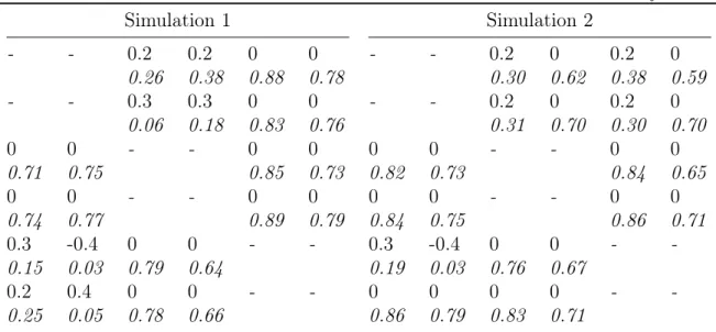
i .13 The same statistics are computed for Σ. Furthermore, the accuracy of the
SSVSP to find the restrictions is evaluated. The posterior probabilities that αlk ij = 0,
ψlk
ij = 0, and αlkjj = αiilk im mean are compared among themselves and in relation
to the true values. These posterior probabilities are calculated as the proportion of γlk
DI,ij, γSI,ijlk , and γCSHw draws that equal zero averaged over all Gibbs sampler draws
and all simulated samples. The higher the proportion ofγ draws that equal zero, the
12The prior hyperparameters used in the Monte Carlo simulations for all different priors are 1.1. 13Koop and Korobilis (2015b) uses the absolute deviation and Korobilis (2016) use the mean absolute
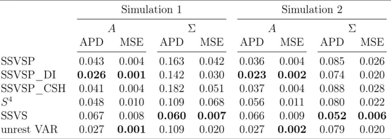
Table 1.1: Deviation for estimated coefficient matrixA and Σfrom the true values
Simulation 1 Simulation 2
A Σ A Σ
APD MSE APD MSE APD MSE APD MSE
SSVSP 0.043 0.004 0.163 0.042 0.036 0.004 0.085 0.026 SSVSP_DI 0.026 0.001 0.142 0.030 0.023 0.002 0.074 0.020 SSVSP_CSH 0.041 0.004 0.182 0.051 0.037 0.004 0.088 0.028 S4 0.048 0.010 0.109 0.068 0.056 0.011 0.080 0.022 SSVS 0.067 0.008 0.060 0.007 0.066 0.009 0.052 0.006 unrest VAR 0.027 0.001 0.109 0.020 0.027 0.002 0.079 0.020
Note: Absolute (APD) and squared (MSE) deviation of the estimates from the true value for co-efficient matrix A and covariance Σ, average over 100 MC draws and all coefficients. Coefficient estimates are the posterior means averaged over all MC draws. Lowest values for each column are in bold. SSVSP_DI: SSVSP with only DI restrictions. SSVSP_CSH: SSVSP with only CSH re-strictions. S4: prior of Koop and Korobilis (2015b). SSVS: prior of George et al. (2008). Unrest
VAR: parameters drawn from unrestricted part of distributions. Simulation 1: DGP has matrix panel structure. Simulation 2: DGP has flexible panel structure.
higher is the probability that no dynamic and no static interdependencies exist and coefficients are homogeneous.
1.5.2 Results
The results of the Monte Carlo study demonstrate that, first, the SSVSP outperforms the S4 in terms of closeness to the true coefficients. This especially holds when a
less restrictive panel structure is present. Second, the SSVSP accurately selects the restrictions for the DGPs of both simulations. This is validated by the higher posterior probabilities for no interdependencies and homogeneity for parameters which are truly zero or homogeneous compared to the probabilities for nonzero and heterogeneous parameters.
As table 1.1 shows, the estimated coefficients which are the posterior means av-eraged over all simulation draws from the SSVSP are on average slightly closer to the true values compared to S4 for both simulations. In particular, the S4
per-forms weaker in simulation 2, where a less restrictive panel structure is present, since the grouping structure on which the restrictions search is done is not present in the data. Furthermore, the APD and MSE of A favor SSVSP_DI for both simula-tions with AP DSSV SP_DI = 0.026 and M SESSV SP_DI = 0.001 for simulation 1 and
AP DSSV SP_DI = 0.023 and M SESSV SP_DI = 0.002 for simulation 2. However, the
unrestricted VAR model outperforms the SSVSP andS4. Doing the restrictions search only for CSH reduces the average deviation from the true values only in simulation 1