e-ISSN: 2278-067X, p-ISSN: 2278-800X, www.ijerd.com
Volume 10, Issue 9 (September 2014), PP.29-37
Current Based Model of Upfc and Dg for Loss Reduction and
Voltage Profile Improvement
B.Raja Rajeswari
1, P.Bhaskara Prasad
2, P.Bala Chennaiah
3 1PG Student, Dept of EEE, Annamacharya Institute of Technology & Sciences, Rajampet, A.P, India 2Assistant Professor, Dept of EEE, Annamacharya Institute of Technology & Sciences, Rajampet, India 3Assistant Professor, Dept of EEE, Annamacharya Institute of Technology & Sciences, Rajampet, India1
[email protected], 2 [email protected], 3 [email protected]
Abstract:- This project shares out with a substitute suggestion for the substantial state modeling of unified power flow controller (UPFC). Since current restrictions are determinant to FACTS apparatus design, the schemed current based model (CBM) assumes the current as variable, allowing easy operation of current restrictions in optimal power flow evaluations. The functioning of the schemed model and of the power injection model (PIM) are compared through a Quasi-Newton escalation approach. Two operating circumstances of a medium size network with 39 busbars were studied from the point of view of escalation and current limits, monitoring the functioning of the UPFC modeling. In general, the electrical power system is a wide variation of a network and it consists of a different equipments such as transmission lines, feeders, transformers, circuit breakers, etc. Due to variations in load or sudden interruption of a network causes to increase in losses and voltage levels of the system are effected. Hence the distributed generation (DG) technology has been paid great attention as far as a potential solution for these problems.
Index Terms:-FACTS, Optimal power flow, Quasi-Newton method, UPFC, CBM, DG
I.
INTRODUCTION
POWER flow studies and escalation techniques are indispensable tools for the safe and economic operation of large electrical systems. The UPFC is one of the most complete apparatus of this new technological family, allowing the regulation of active and reactive powers, substantially enlarging the operative flexibility of the system.[1]-[5]
Substantial state models of UPFC illustrated in the literature employ the power balance equation, resulting in the impartiality of the series and shunt active power of converters assuring no internal active power consumption or generation.
One of the first schemed models[6] uses this condition, but only in particular cases, when power and voltage are admittedly known, is the implementation of the model in conventional power flow program viable.
The employed models [7] in represent the active elements through equivalent passive circuits, including the power balance equation. In the passive model consists of a susceptance and an ideal voltage transformer and the fundamental power balance equation is intrinsically included. Voltage source models employed in [8]-[10] consist of series and shunt voltages offered in the equations as control variables.
The model illustrated[11], known as power injection model (PIM), is quite spread in the literature, representing the effect of active elements by equivalent injected powers. In the traditional models, the current is not clearly treated in the equations. As in the design of FACTS converters one of the main limitations lies on current limitation, it is expedient to have a model that uses the current as a variable, which will be the purpose of this paper.
II.
CURRENT BASED MODEL
The developed model signifies the UPFC in substantial state, introducing the current in the series converter as variable
1). Series voltage
2) Transformer impedance
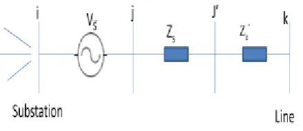
Fig. 1. UPFC and network.
Let us consider busbars i and k existent in the transmission line where the UPFC will be located, with impedance. Busbars j and j’ are created in order to include the UPFC in the system. The series impedance of UPFC coupling transformer and the transmission line are added, resulting in the equivalent impedance connected to the internal node and node is eliminated. This alliance is quite simple, even in case of two port lines reoffered by π circuits.
The equivalent network is offered in Fig. 2, with the series voltage inserted between busbars i and j
Fig. 2. Equivalent model of UPFC in the electric network.
Fig. 3. Injected power due to current in busbars.
A. Injected Power Due to Current
The power intake of the system load at bus bar is called Si 0
.Additional powers, due to current, are easily calculated according to Fig. 3. Current introduces two variables, related to module and phase of the current. We can write the new power expressions due to current:
S
ic= V
iI
*S
jc= -V
jI
*(1)
P
ic= V
iI cos 𝜑 − 𝜃
𝑖P
jc= −V
jI cos
(𝜑 − 𝜃
𝑗)
(2)
Q
ci= V
iI sin 𝜑 − 𝜃
𝑖Q
cj= −V
jI sin
(𝜑 − 𝜃
𝑗)
(3)
We have
𝑃
𝑖= 𝑃
𝑖0+ 𝑃
𝑖𝑐𝑃
𝑗= 𝑃
𝑗𝑐(4)
𝑄
𝑖= 𝑄
𝑖0+ 𝑄
𝑖𝑐𝑄
𝑗= 𝑄
𝑗𝑐(5)
Placing the new variables and at and position, respectively, the new vector of variables can be written
𝑥
𝑡= 𝜃
1
, 𝜃
2, . 𝜃
𝑛 −1,𝜑, 𝑉
1, 𝑉
2, … 𝑉
𝑛−1, 𝐼
(6)
B. Series Voltage Equations
The following treatment of the series voltages for the UPFC is general for FACTS devices that can employ this feature. The main example is the SSSC and, as a consequence, other apparatus such as IPFC and GIPFC that use series voltage can be modeled as well. Writing the voltage equation between nodes and we obtain
The series voltage will be treated similarly to the PIM model of:
𝑉
𝑠= 𝑟𝑣
𝑖𝑒
𝑗𝛿(8)
Where r is the factor for series voltage and is the series voltage angle. That equation substituted in (7) results
𝑣
𝑗− 1 + 𝑟𝑒
𝑗𝛿𝑣
𝑖
= 0
(9)
If r and δ are constants, in a regular power flow case, calling the complex variable
𝐴∠𝛼 = −(1 + 𝑟∠𝛿)
(10)
𝑣
𝑗+ 𝐴∠𝛼𝑣
𝑖= 0
(11)
We obtain the equations, relative to the real and imaginary parts and, respectively:
𝐹
𝑛= 𝐴𝑉
𝑖cos( 𝛼 + 𝜃
𝑖) + 𝑉
𝑗𝑐𝑜𝑠𝜃
𝑗(12)
𝐺
𝑛= 𝐴𝑉
𝑖sin 𝛼 + 𝜃
𝑖+ 𝑉
𝑗𝑠𝑖𝑛𝜃
𝑗(13)
These equations will be put at the end of the equation system. If r and del are variables in an escalation case, we have
𝑥
𝑡= 𝜃
1
, 𝜃
2, … 𝜃
𝑛 −1,𝜑, 𝛿, 𝑉
1, 𝑉
2, … … 𝑉
𝑛−1, 𝐼, 𝑟
(14)
𝐹
𝑛= 𝑉
𝑗cos( 𝜃
𝑗) − 𝑉
𝑖[cos 𝜃
𝑖+ cos 𝜃
𝑖+ 𝛿 ] (15)
𝐺
𝑛= 𝑉
𝑗sin 𝜃
𝑖− 𝑉
𝑖[sin 𝜃
𝑖+ sin 𝜃
𝑖+ 𝛿 ]
(16)
C. Power Balance
In order to complete the UPFC model, it is necessary to introduce the power balance equation between series and shunt converters. The series power will be added to the shunt power of bus bar, similarly (see Fig. 4).
Fig4:Injected powers in the busbars with the inclusion of UPFC.
Let us calculate the power in the series converter:
𝑆
𝑠= 𝑟𝑒
𝑗𝛿𝑉
𝑖𝐼⦞ − 𝜑)
(17)
Splitting the previous expression in active and reactive powers:
𝑃
𝑠= 𝑟𝑉
𝑖𝐼𝑐𝑜𝑠(𝜃
𝑖+ 𝛿 − 𝜑)
(18)
𝑄
𝑠= 𝑟𝑉
𝑖
𝐼𝑠𝑖𝑛(𝜃
𝑖+ 𝛿 − 𝜑)
(19)
D. Complete Jacobean
Calling the Jacobean matrix, without UPFC power addition
𝐽
𝑐0=
𝐻
0
𝑁
0𝐽
0𝐿
0(20)
Let us add the injected power due to current in busbars and also the voltage equations. The additional correction of the Jacobean matrix, due to the power balance equation, is also included, complementing the formulation
𝐽 = 𝐽𝑐0 + 𝐽𝑐 + [𝐽𝑠]
(21)
E. Escalation Approach
The behavior of the schemed model was studied with an escalation power flow code based on the Quasi-Newton method. The Quasi-Newton method was used in order to compare time answers of PIM and CBM models, adopting the same initial conditions and trying to obtain similar results as possible, although some differences in the equations of both cases can lead to small discrepancies in some variables of the system. The approximation formula used in the Quasi-Newton method is given by [12] and [14]
𝐸𝑘 +1 = 𝐼𝑑 − 𝑝𝑘𝑦𝑘𝑇
𝑝𝑘𝑇𝑦𝑘 𝐸𝑘 𝐼𝑑− 𝑦𝑘𝑇𝑝𝑘
𝑝𝑘𝑇𝑦𝑘 + 𝑝𝑘𝑝𝑘𝑇
𝑝𝑘𝑇𝑦𝑘
(22)
Where
𝐸𝑘 +1=inverse of approximation of Taylor series expansion of the gradients of f in 𝑥𝑘+1
𝑝𝑘= 𝐸𝑘+ 𝑗𝑦𝑘 secant relationship or Quasi Newton
Yk = Taylor series expansion (∇f𝑥𝑘 +1-∇f𝑥𝑘)
𝐼𝑑 = Identity matrix
Current restrictions are introduced in the formulation. In the CBM, current module and angle are the variables of the problem, while for PIM current equation is introduced according to
Ī = 𝑉
𝑖⦟𝜃
𝑖+ 𝑟𝑉
𝑖⦟ 𝜃
𝑖+ 𝛿 − 𝑉
𝑗⦟𝜃
𝑗(𝑗𝑏
𝑠)
(23)
Equation (23) would be a little more complex if the series admittance was not simplified to disregarding series impedance losses.
III. RESULTS
Several comparative tests performed with CBM and PIM models offered identical results in power flow analysis using a MATLAB code. An additional comparison with the model of was made, using the Power World program.
Some modifications in the New England System of 39 bus-bars were introduced with the purpose of highlighting the optimization results. Generator 2 is the swing bus bar, and the other generators are considered power variable generators and generation costs are also offered. In the modified network, the base case does not converge and convergence can only be attained if the power generation cost is optimized. If current restrictions are used in some lines, convergence is only attained with UPFCs in the network.
Voltage results were considered inside the range 0.95 to 1.05 pu for network busbars. In order to make a fair comparison
By the UPFC the power losses are considerably high so for reducing the power losses introducing the DGs to this network. For the allocation of DG here we are considering the voltage constrains and losses are consider for the size of the DG the improved performance is also presented for both 3 UPFC model and 6 UPFC models.
A. Network with 3 UPFCs
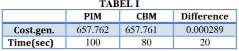
With 3 UPFCs, despite the higher Jacobean dimension of CBM, its convergence time is lower since restrictions on current treated as a variable enable fast convergence. Most variables such as voltage, current and angle obtained in the convergence of three UPFCs are identical in both models, but this is not true if current limits are increased. Reducing the current band limits, PIM does not usually converge. The same generation cost offered by the two models and the lower computation time of the CBM model can be verified this is presented in table I.
TABEL I
PIM CBM Difference
Cost.gen. 657.762 657.761 0.000289
Time(sec) 100 80 20
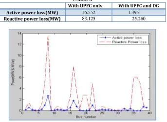
Before placement of DG the active and reactive power losses are 16.552Mw 83.125Mvar.After placement of DG the losses are reduced to 1.395Mw and 25.260 MVAR respectively. The bus wise losses without and with DG placement are shown in in fig.5 and fig.6 respectively.
TABLE II
With UPFC only With UPFC and DG
Active power loss(MW) 16.552 1.395
Reactive power loss(MW) 83.125 25.260
Fig.5. power losses without DG placement
Fig.6. power losses with DG placement
B. Network with 6 UPFCs
By increasing the number of UPFCs to 6, the lower convergence time of CBM is still more evident. The results of the variables of the two models are not similar but generation costs are almost the same for these limits. If the limits are increased, different generation costs can be yielded for the models.the cost generation with two models are shown in tabel II.
TABEL III
PIM CBM Difference
Cost.gen. 518.649 518.631 0.003
Time(sec) 100 80 20
presenting a better functioning in cases of difficult convergence due to current restrictions, mainly in cases with narrower current limits.
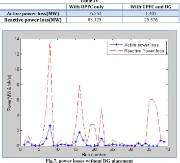
With the 6 upfcs Before placement of DG the active and reactive power losses are 16.552Mw and 83.125 Mvar After placement of DG the losses are reduced to 1. .405Mw and 25.576 Mvar. The bus wise losses without and with DG placement are shown in in fig.7 and fig.8 respectively
Table IV
With UPFC only With UPFC and DG
Active power loss(MW) 16.552 1.405
Reactive power loss(MW) 83.125 25.576
Fig.7. power losses without DG placement
Fig.9 Modified England network with 6 UPFC
IV.
CONCLUSION
This paper presents the treatment of series voltage converters in power systems and the formulation can be useful to other apparatus of the FACTS family. The suggestion of a substitute formulation for the modeling of UPFC was offered, considering the current in the series converter as a variable. The proposed CBM model was compared with the conventional power injection model PIM, showing coincident results in power flow evaluations.
In an escalation approach, despite carrying out with two additional equations for each UPFC, the CBM model reduces the computational time, when current restrictions are introduced in the series converters, mainly when dealing with several UPFC in the system, which is a very important issue in FACTS design.
Distributed generations (DGs) are placed to minimize the total power loss of system. Depending on the voltage constraints the dg location was found. The proposed procedure based on the UPFC and DG took the only few samples, and therefore reduced the computational requirement dramatically during the optimization process.
APPENDIX
H terms :
𝐻
𝑖𝑖𝑐=
𝜕𝑃𝑖𝑐 𝜕𝜃𝑖= −𝑄
𝑖 𝑐𝐻
𝑗𝑗𝑐=
𝜕𝑃𝑗𝑐 𝜕𝜃𝑗= −𝑄
𝑗 𝑐𝐻
𝑖𝑛𝑐=
𝜕𝑃𝑖𝑐 𝜕𝜑= −𝑄
𝑖 𝑐𝐻
𝑗𝑛𝑐=
𝜕𝑃𝑗𝑐 𝜕𝜑= −𝑄
𝑗 𝑐𝐻
𝑛𝑖= −𝐴𝑉
𝑖sin(𝛼 + 𝜃
𝑖) 𝐻
𝑛𝑗= −𝑉
𝑗sin(𝜃
𝑗)
N terms:
𝑁
𝑖𝑖𝑐= 𝑉
𝑖𝜕𝑃𝑖𝑐 𝜕𝑉𝑖= 𝑃
𝑖 𝑐𝑁
𝑗𝑗𝑐= 𝑉
𝑗 𝜕𝑃𝑗𝑐 𝜕𝑉𝑗= 𝑃
𝑗 𝑐𝑁
𝑖𝑛𝑐= 𝐼
𝜕𝑃𝑖𝑐 𝜕𝐼= 𝑃
𝑖 𝑐𝑁
𝑛𝑗𝑐= 𝐼
𝜕𝑃𝑖𝑐 𝜕𝜑= 𝑃
𝑗 𝑐𝑁
𝑛𝑖= 𝐴𝑉
𝑖cos(𝛼 + 𝜃
𝑖) 𝑁
𝑛𝑗= 𝑉
𝑗cos(𝜃
𝑗)
J terms:
𝐽
𝑖𝑖𝑐=
𝜕𝑄𝑖𝑐 𝜕𝜃𝑖= 𝑃
𝑖 𝑐𝐽
𝑗𝑗𝑐=
𝜕𝑄𝑗𝑐 𝜕𝜃𝑗= 𝑃
𝑗 𝑐𝐽
𝑖𝑛𝑐=
𝜕𝑄𝑖𝑐 𝜕𝜑= −𝑃
𝑖 𝑐𝐽
𝑗𝑛𝑐=
𝜕𝑄𝑗𝑐 𝜕𝜑= −𝑃
𝑗 𝑐𝐽
𝑛𝑖= 𝐴𝑉
𝑖cos(𝛼 + 𝜃
𝑖) 𝐽
𝑛𝑗= 𝑉
𝑗cos(𝜃
𝑖)
L terms:
𝐿
𝑐𝑖𝑖= 𝑉
𝑖 𝜕𝑄𝑖𝑐 𝜕𝜃𝑖= 𝑄
𝑖 𝑐𝐿
𝑗𝑗 𝑐= 𝑉
𝑗 𝜕𝑄𝑗𝑐 𝜕𝜃𝑗= 𝑄
𝑗 𝑐𝐿
𝑐𝑖𝑛= 𝐼
𝜕𝑄𝑖𝑐 𝜕𝐼= 𝑄
𝑖 𝑐𝐿
𝑖𝑛 𝑐= 𝐼
𝜕𝑄𝑗𝑐 𝜕𝜑= 𝑄
𝑗 𝑐𝐿
𝑛𝑖= 𝐴𝑉
𝑖sin(𝛼 + 𝜃
𝑖) 𝐿
𝑛𝑗= 𝑉
𝑗sin(𝜃
𝑗)
Correction in Jacobean terms due to power balance
H terms:
𝐻
𝑖𝑖𝑠=
𝜕𝑃𝑠𝜕𝜃𝑖
= −𝑟𝑉
𝑖sin(𝜃
𝑖+ 𝛿 − 𝜑) = −𝑄
𝑠
𝐻
𝑖𝑛𝑠=
𝜕𝑃𝑠𝜕𝜑
= 𝑟𝑉
𝑖sin(𝜃
𝑖+ 𝛿 − 𝜑) = 𝑄
𝑠
N terms:
𝑁
𝑖𝑖𝑠= 𝑉
𝑖𝜕𝑃𝑠𝜕𝑉𝑖
= 𝑟𝑉
𝑖𝐼 cos(𝜃
𝑖+ 𝛿 − 𝜑) = 𝑃
𝑠𝑁
𝑖𝑛𝑠= 𝐼
𝜕𝑃𝑠𝜕𝐼
= 𝑟𝑉
𝑖𝐼 cos(𝜃
𝑖+ 𝛿 − 𝜑) = 𝑃
𝑠[H] sub –matrix terms
𝐻
𝑖𝑖= 𝐻
𝑖𝑖0− 𝑄
𝑖𝑐− 𝑄
𝑠𝐻
𝑗𝑗= 𝐻
𝑗0− 𝑄
𝑗𝑐𝐻
𝑖𝑛= 𝑄
𝑖𝑐+ 𝑄
𝑠𝐻
𝑗𝑛= 𝑄
𝑗𝑐𝐻
𝑛𝑖= −𝐴𝑉
𝑖sin(𝛼 + 𝜃
𝑖) 𝑁
𝑛𝑗= −𝑉
𝑗sin(𝜃
𝑗)
[N] sub matrix terms
𝑁
𝑖𝑖= 𝑁
𝑖𝑖0+ 𝑃
𝑐𝑖+ 𝑃
𝑠𝑁
𝑗𝑗= 𝑁
𝑗𝑗0+ 𝑃
𝑗𝑐𝑁
𝑖𝑛= 𝑃
𝑖𝑐+ 𝑃
𝑠𝑁
𝑗𝑛= 𝑃
𝑗𝑐𝑁
𝑛𝑖= 𝐴𝑉
𝑖cos(𝛼 + 𝜃
𝑖) 𝑁
𝑛𝑗= 𝑉
𝑗cos 𝜃
𝑗[J] Sub matrix terms
𝐽
𝑖𝑖= 𝑃
𝑖0+ 𝑃
𝑖𝑐𝐽
𝑗𝑗= 𝐽
𝑗𝑗0+ 𝑃
𝑗𝑐𝐽
𝑖𝑛= −𝑃
𝑖𝑐𝐽
𝑗𝑛= −𝑃
𝑗𝑐[L] Sub matrix terms
𝐿
𝑖𝑖= 𝐿
0𝑖𝑖+ 𝑄
𝑖𝑐𝐿
𝑗𝑗= 𝐿
𝑗𝑗0+ 𝑄
𝑗𝑐𝐿
𝑖𝑛= 𝑄
𝑖𝑐𝐿
𝑗𝑛= 𝑄
𝑗𝑐𝐿
𝑛𝑖= 𝐴𝑉
𝑗sin(𝛼 + 𝜃
𝑗) 𝐿
𝑛𝑗= 𝑉
𝑗sin(𝜃
𝑗)
REFERENCES
[1]. N.G.Hingorani and L. Gyugyi, Understanding FACTS: Concepts and Technology of Flexible AC Transmission Systems. New York: IEEEPress, 2000.
[2]. J. Bian, D. G. Ramey, R. J. Nelson, and A. Edris, “A study of apparatus sizes and constraints for a unified power flow controller (UPFC),” IEEETrans. Power Del., vol. 12, no. 3, pp. 1385–1391, Jul. 1997.
[3]. K. K. Sen and E. J. Stacey, “UPFC-unified power flow controller: Theory, modeling and applications,”
IEEE Trans. Power Del., vol. 13, no. 4, pp. 1953–1960, Oct. 1998.
[4]. F. Keri et al., “Unified power flow controller (UPFC): Modeling and analysis,” IEEE Trans. Power Del., vol. 14, no. 2, pp. 648–654, Apr. 1999.
[5]. L. Gyugyi, C. Schauder, and K. K. Sen, “Static synchronous series compensator: A solid state approach to the series compensation of transmission lines,” in Proc. IEEE Transmission & Distribution Conf., 96-Winter Meeting, Baltimore, MD, 1996.
[6]. M. R. Iravani and A. Nabavi-Niaki, “Substantial-state and dynamic models of unified power flow controller (UPFC) for power system studies,” IEEE Trans. Power Syst., vol. 11, no. 4, pp. 1937–1943, Nov. 1996.
[7]. L. Lábbate,M. Trovato, C. Becker,and H. Andschin, “Advancedsubstantial-state models of UPFC for power systems studies,” in Proc. IEEE PESSummer Meeting, Chicago, IL, Jul. 2002, vol. 1, pp. 449– 454.
[8]. C. R. Fuerte-Esquivel and E. Acha, “Newton-Raphson algorithm for the reliable solution of large power networks with embedded FACTS devices,” Proc. Inst. Elect. Eng., Gen., Transm., Distrib., vol. 143, no. 5, pp. 447–454, Sep. 1996.
[9]. C. R. Fuerte-Esquivel and E. Acha, “Unified power flow controller: A critical comparison of Newton-Raphson UPFC algorithms in power flow studies,” Proc. Inst. Elect. Eng., Gen., Transm., Distrib., vol. 144, no. 5, pp. 437–444, Sep. 1997.
[10]. C. R. Fuerte-Esquivel, E. Acha, and H. Ambriz-Perez, “A comprehen-sive Newton-Raphson UPFC model for the quadratic power flow so-lution of practical power networks,” IEEE Trans. Power Syst., vol. 15, no. 1, pp. 102–109, Feb. 2000.
[11]. M. Noroozian and G. Andersson, “Power flow control by use of con-trollable series components,”
IEEE Trans. Power Del., vol. 8, no. 3, 1420–1429, Jul. 1993.
[12]. K. M. Soon and R. H. Lasseter, “A Newton-type current injection model of UPFC for studying low-frequency oscillations,” IEEE Trans.Power Del., vol. 19, no. 2, pp. 694–701, Apr. 2004.
[13]. J. E. van Ness and J. H. Griffin, “Elimination methods for load flow studies,” Trans. Power App. Syst., vol. PAS-80, pt. III, pp. 229–304, 1961.
[14]. D. F. Shanno, “Conditioning of Quasi-Newton methods for function minimization,”