State space control using LQR method for a cart-inverted pendulum
linearised model
Indrazno Siradjuddin
1, Budhy Setiawan
1, Ahmad Fahmi
2, Zakiya Amalia
1and Erfan Rohadi
3 1Electrical Engineering Department, Malang State Polytechnic, Malang, Indonesia2Electrical Engineering Department, Malang State University, Malang, Indonesia 3Information Technology Department, Malang State Polytechnic, Malang, Indonesia
The Cart-Inverted Pendulum System (CIPS) is a classical benchmark control problem. Its dynamics resembles with that of many real world systems of interest like missile launchers, pendubots, human walking and segways and many more. The control of this system is challenging as it is highly unstable, highly non-linear, non-minimum phase system and underactuated. Furthermore, the physical constraints on the track position also pose complexity in its control design. This paper presents a control method to stabilise the unstable CIPS within the different physical constraints such as in track length and control voltage. A novel cart-inverted pendulum model is proposed where mechanical transmission and a dc motor mathematical model have been included which resembles the real inverted pendulum. Therefore problems emerged in realtime implementation can be minimised. A systematic the state feedback design method by choosing weighting matrices key to the Linear Quadratic Regulator (LQR) design is presented. Simulation experiments have been conducted to verify the controller’s performances. From the obtained simulation and experiments it is seen that the proposed method can perform well stabilising the pendulum at the upright angle position while maintaining the cart at the desired position.
Index Terms—Cart-Inverted Pendulum, Linear Quadratic Regulator, Optimal Control, Non Linear System
I. INTRODUCTION
C
ONTROLLING a Cart-Inverted Pendulum System (CIPS) is a challenging problem which is widely used as benchmark for testing control algorithms such as PID controllers [1], neural networks [2], [3], fuzzy control [4], genetic algorithms [5]. The CIPS features as higher order, nonlinear, strong coupling and multivariate system, which has been studied by many researchers. It is used to model the field of robotics and aerospace field, and so has important significance both in the field of the theoretical study research and practice. It has good practical applications right from mis-sile launchers to segways, human walking, earthquake resistant building design etc. The CIPS dynamics resembles the missile or rocket launcher dynamics as its center of gravity is located behind the centre of drag causing aerodynamic instability. The CIPS has two equilibrium points [6], one of them is stable while the other is unstable. The stable equilibrium corresponds to a state in which the pendulum is pointing downwards. The control challange is to maintain the pendulum at the unstable equilibrium point where the pendulum upwards, with minimum control energy. In recent times optimal control provides the best possible solution to process control problems for a given set of performance objectives. Detail review on optimal control has been presented in [7]. Survey on optimal control approaches and their applications have been conducted, for instance, an optimal control approach for inventory systems [8] and energy optimisation [9].This paper investigates the application of the Linear Quadratic Regulator (LQR) to stabilise the CIPS at the unsta-ble equilibrium point. The organisation of this paper is struc-tured as follows: The dynamic modelling using Lagrangian Corresponding author: Indrazno Siradjuddin (email: [email protected]).
approach firstly discussed in Section II In this section, the state space representation of the CIPS is presented where the DC motor and its transmission system are considered. Section III discusses the LQR method in detail, followed by simulation and results of the LQR control approach applied on CIPS problem presented in Section IV Conclusion is presented in Section V
II. SYSTEMMODELING A. Lagrange’s Equation
Lagrange’s equation is used to describe the motion equation of a complex system dynamic in a very efficient way. It reduces the need for complicated vector analysis that usually required for discribing forces applied on a mechanical system.
The fundamental principle of Lagrane’s equation is the representation of the system by a set of generalised coordinate q = {q1,· · ·, qi,· · ·, qn}, where n is the total assigned
generalised coordinate.qiis an independent degree of freedom
of true system which completely incorporate the contraints unique to that system, i.e., the interconnections between parts of the system.
The Lagrangian function L is expressed by the kinetic energy Kand the potential energy P as discribed as follows
L=K(q,q)˙ − P(q) (1)
where the kinetic energy function in terms of the geralised coordinateqand its derivativeq. The potential energy function˙ is expressed in terms of only the generalised coordinate.
The desired motion equations are derived using d
dt
∂L
∂q˙i
−∂L ∂qi
where Qi denotes the external force applied in term of qi
coordinate. The expression in (2) is called Lagrange’s equa-tion. It can be deduced that for ngeneralised coordinates, the system dynamic is represented byn second order differential equations.
B. Lagrange’s Equation of The System
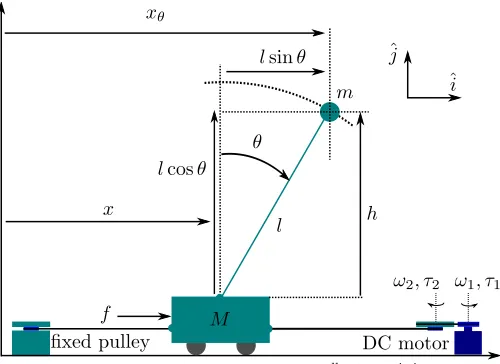
Fig. 1. The inverted pendulum on a cart system
The motion of the cart is only inˆi direction, thus the total kinetic energy of the cart can be expressed as
KM =
1 2Mx˙
2 (3)
The pendulum moves inˆj andˆidirections, therefore the total kinetic energy of the pendulum is expressed as
Km=
1
2m( ˙xθ+ ˙h) (4) It can be seen in Fig. 1 that
xθ = x+lsinθ (5)
h = lcosθ (6)
Taking the derivative of Eq. (5) and Eq. (6), we have ˙
xθ = x˙+lθ˙cosθ (7)
˙
h = −lθ˙sinθ (8)
Therefore, the pendulum kinetic energy in Eq. (4) can be rewritten as
Km =
1
2m(( ˙x+l ˙
θcosθ)2+ (−lθ˙sinθ)2) (9) = 1
2m( ˙x
2+ 2 ˙xlθ˙cosθ+l2θ˙2) (10)
hence the total kinetic energy from the cart and the pendulum can be obtained as
K = KM +Km (11)
= 1 2Mx˙
2+1
2m( ˙x
2+ 2 ˙xlθ˙cosθ+l2θ˙2) (12)
The potentioal energy involved in the system is only from the pendulum massm
P = mgh (13)
= mglcosθ (14) Then, the Lagrangian equation (15) can be fully defined using Eq. (12) and Eq. (14), as follows
L = 1
2Mx˙
2+1
2m( ˙x
2+ 2 ˙xlθ˙cosθ+l2θ˙2)
−mglcosθ (15)
The motion of the inverted pendulum on a cart can be specifi-cally defined by the displacement of the cart in theˆidirection with respect to the origin and the angle of the pendulum with respect to the ˆj direction. Hence, the system only has two degrees of freedom reprented byxandθ, the system dynamics must be expressed in terms ofxandθ. Thus,xandθ can be selected as the elements of the generalised coordinate vector q. Using this selection, the Lagrange’s equation (??) can be expressed for each generalised coordinate:
d dt
∂L
∂x˙
−∂L
∂x = f (16)
d dt
∂L
∂θ˙
−∂L
∂θ = 0 (17)
It is assumed that the external forces applied on the system is only applied on cart in ˆi direction, there is no external torque applied on the pendulum. Deriving for each term in the differential equation in (16) and (17), it can be obtained that
∂L
∂x˙ = (M +m) ˙x+ml ˙
θcosθ (18) d
dt
∂L ∂x˙
= (M +m)¨x+mlθ¨cosθ
−mlθ˙2sinθ (19)
∂L
∂x = 0 (20)
and
∂L
∂θ˙ = mlx˙cosθ+ml
2θ˙ (21)
d dt
∂L ∂θ˙
= ml(¨xcosθ−θ˙x˙sinθ)
+ml2θ¨ (22)
∂L
∂θ = −mxl˙
˙
θsinθ+mglsinθ (23) Therefore, the Lagrange’s equation for each generalised coor-dinate can be rewritten as
f = (M+m)¨x+mlθ¨cosθ−mlθ˙2sinθ (24) 0 = ml(¨xcosθ−θ˙x˙sinθ) +ml2θ¨
θ,sinθ ≈θ andcosθ≈1. Deriving Eq.(24) and (25) using this approximation, one will find the quadratic terms θ˙2 and
˙
θθ. In the small region near equilibrium, the termsθ˙2 andθθ˙ are significantly small. Using aforementioned assumptions, the linearised Lagrange’s equation can be obtained as follows
f = (M +m)¨x+mlθ¨ (26) 0 = x¨+lθ¨−gθ (27)
C. DC Motor: Torque, Armature Voltage and Angular Ve-locity Model
The armature circuit equation is
iaRa+La
dia
dt +vb = va (28)
The generated back electromotive force (emf),vb, is
propor-Fig. 2. DC Motor Armature Equivalent Circuit tional to the rotational speed of the rotor
vb = Kb
dθ1
dt (29)
whereKb is the back emf constant andω1=dθdt1. The motor
torque τ1 is proportional to the armature current ia, hence
τ1 = Ktia (30)
where Kt is the motor torque constant. Substituting Eq.(29)
and (30) (in term of ia) into (28), one obtains
τ1
Kt
R+La
d2τ 1
(dt)2 +Kb
dθ1
dt = va (31)
Generally, the inductor in the rotor is small, thus can be neglected, then the armature circuit equation in term of τ1
becomes
τ1 = −Kt
Kb
Ra
ω1+
Kt
Ra
va (32)
In the mechanical transmission (i.e., geared and pulley sys-tems), it applies a following formula
τ2
τ1
= N2
N1
= ω1
ω2
=r2
r1
(33) whereN is the number of a gear teeth andris the radius of a pulley. The motor angular velocity ω1 can be expressed in
term of the cart velocity x˙ (reffering to the Fig.1) by 2πr2
˙
x =
r2
r1
2π ω1
(34)
where the term 2πr2 is the circumference of the pulley that
connects to the cart using a belt. Therefore,
ω1=
˙
x r1
(35) Substituting Eq.(35) into Eq.(32) yields
τ1 = Kr(−Kb
˙
x r1
+va) (36)
The force that moves the cart is caused by the torque τ2, for
this reason, it is needed to transformτ17→τ2. Consequently,
using f r2=τ2 (the force that perpendicular to the direction
of r2 from pulley centre), it can be verified that
f =Kr
r1
(−Kb
˙
x r1
+va) (37)
whereKr = KtRa. Substituting Eq.(37) into Eq.(26) produces
a new Lagrange’s equation in term of generalised coordinate
xas follows
Kr
r1
va = (M+m)¨x+
KrKb
(r1)2
˙
x+mlθ¨ (38) To simplify the derivation, the following shorthands are used
c1 =
KrKb
(r1)2
(39) c2 =
Kr
r1
(40) then from the Lagrange’s equation (38), and by substituting the term lθ¨from Eq.(27) into Eq.(38), it can be obtained a following the first differential equation of the system
¨
x = 1
M (c2va−c1x˙−mgθ) (41)
Rearranging Eq.(27), one can derive ¨
θ = 1
l (gθ−x¨) (42)
Substituting Eq.(41) into Eq.(42), the second differential equa-tion of the system can be expressed as follows
¨
θ = 1
l
gθ− 1
M (c2va−c1x˙−mgθ)
(43)
= −c2 M lva+
c1
M lx˙+
(M+m)g
M l θ (44)
At this point, the diffrential equations of the cart-pendulum motion which based on the Lagrange’s method have been developed. Next step, before the optimal controller can be defined, firstly, the differential equations in the state space representation has to be formed, as discussed in the following section.
D. State Space Representation
Following equations are state space representation of a system ˙
x = Ax+Bu (45)
y = Cx+Du (46)
wherex ∈Rj is a state vector and j is the total number of
Fig. 3. Open loop system
A vector u∈Rk is the control input or control vector which
has k elements of control variables. The A ∈ Rj×j, B ∈ Rj×k andC∈Rp×j are called the system, the input and the
output matrices, respectively, where p is the output number. The output vector is denoted asy∈Rp. The open loop system
diagram describing the state space form is shown in Fig.3. For the case of CIPS, the state vector, its derivative and the control input are defined as x = [x θx˙θ˙]T,x˙ =
[ ˙xθ˙¨xθ¨]T, u = v
a, respectively. Composing Eq.(41) and
Eq.(44) into the state space form, we have
A =
0 0 1 0
0 0 0 1
0 −mgM −c1
M 0
0 (M+m)gM l c1
M l 0
,
B =
0 0
c2 M
−c2 M l
,C=
1 0 0 0 0 1 0 0
y = [x θ]T,D=∅
It is assumed that onlyxandθcan be observed from sensors (e.g optical encoders) and the mapping from the state vector into the output vector is one-to-one mapping.
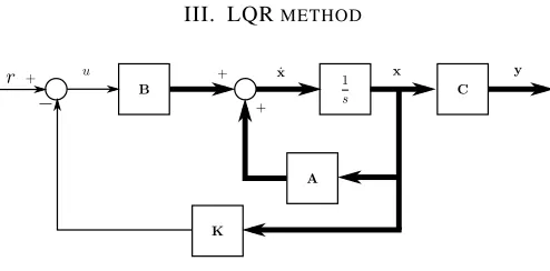
III. LQRMETHOD
Fig. 4. Closed loop system
Linear Quadratic Regulator Controller is based on full state-feedback control principle (see Fig.4). The control gain K can be obtained, based on minimising the perfomance cost function described as
J = ∞
Z
0
(xTQx+u2R)dt (47)
whereQ∈Rj×j is a real symmetric matrix andRis a scalar
that both should be selected. QandRdetermine the relative
importance of the error and the energy cost. Therefore, the matrix Q and R signify the trade-off between performance and control effort respectively. If|Q|is relatively smaller than
R, the control system becomes expensive sinceJ primarily penalises the use of control energy. In contrast, when|Q| is relatively bigger thanR, the control system becomes a cheap control because an arbitrary small control effort can be used to stabilise the system, however, the system responses will be relatively slow. It is a common practice to letR>0 and Q
be a diagonal matrix in the form of
Q =
q1 0 · · · 0
0 q2 · · · 0
..
. ... . .. 0 0 0 · · · qj
(48)
where (q1, q2,· · ·, qj) are positive values. From the Laplace
transfer function of the closed loop system (Fig,4), the denom-inator can be found as
D(s) =sI−(A−BK) (49)
where I is an identity matrix. Hence, all eigenvalues of (A −BK) determine the stability and transient response characteristics of the closed loop system. The design effort is to select the feed-back gainK such that the eigenvalues of (A−BK)have negative real parts. The optimal feed-back gain Kcan be obtained by solving the following Riccati Equation for a positive definite matrixP:
ATP+PA−PBR−1BTP+Q = 0 (50) then the optimal feed-back gainK can be computed as
K =R−1BTP (51)
Note that if matrix (A−BK) is a stable matrix then P always exists. In contrast, for the case of an unstable matrix (A−BK), the matrix Pdoes not exist for solving Eq.(50). Thus, it is necessary for the control engineer to check the con-trollability and observability of the system model beforehand the controller implementation. The controllability means that for any initial state values, the acceptable control effortucan steer the state to any final state values within some finite time window if only if rank(C) is equal to the number of state variables.
C =
A|AB|A2B| · · · |Aj−1B
(52)
rank(C) = j (53)
Observability is a property of the plant with appropriate sensor selection without considering actuator selection. To test that the system is an observable system, the rank of observability matrix Ohas to be equal to the number of the state. The observability matrixOcan be computed as
O =
C|CA|CA2| · · · |CAj−1
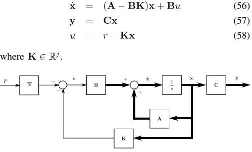
unsastifactory dc gain N,0 < N < 1. The transfer function of a closed loop system shown in Fig.4 is expressed as
T(s) =C(sI−(A−BK))−1B (55) where dc gain N can be obtained by T(s)|s=0. The solution
to improve the performance of the steady state error is to put a pregain N¯ in the system as depicted in Fig.5. The pregain
¯
N is computed as N¯ =N1. The full state space equation can be expressed as
˙
x = (A−BK)x+Bu (56)
y = Cx (57)
u = r−Kx (58)
whereK∈Rj.
Fig. 5. Closed loop system with pregain
IV. SIMULATION ANDRESULTS
In order to simulate the full state feed-back control system, the defined system parameters in Table I are used. The resulting eigenvalues of the open loop system depicted in Fig.3 are {0,6.5681,−6.5718,−0.0364} which can be obtained by det(sI−A). It can be seen that the open loop system has a positive real part, therefore, the system is an unstable system. However, using the system state space described in Eq.(45) and (46), the CIPS is a completely controllable and observable since the matrix ranks ofCandOare both equal to the number of the state, rank(C) = rank(O) = 4, which can be verified using results shown in Eq.(59) and Eq.(60).
TABLE I THECIPSPARAMETERS
No. Parameter Value Units
(1) Ra 1 Ω
(2) Kt 0.02 N·m/A
(3) Kb 0.02 V·s/rad
(4) r1 0.015 m
(5) M 1 Kg
(6) m 0.1 Kg
(7) l 0.25 m
C=
0 0.200 −0.008 0.785 0 −0.800 0.032 −34.533 0.200 −0.008 0.785 −0.063
−0.800 0.032 −34.533 1.507
(59)
O=
1 0 0 0
0 1 0 0
0 0 1 0
0 0 0 1
0 −0.981 −0.040 0 0 43.164 0.160 0 0 0.039 0.002 −0.981 0 −0.157 −0.006 43.164
(60)
The first design choice of Q andRin the performance cost function are Q=CTC=diag{1,1,0,0} andR= 1. It can be noted that the elements of matrix Q; {q1, q2} = {1,1}
means that the design choice control effort tries to make an equal emphasis between statexandθregardles the condition of statex˙ andθ˙. Furthermore, the initial choice ofQensures that xTQx is a positive semi definite matrix, for all x. The
feedback gainK, the characteristic polynomial functionD(s) and its roots are found as follow
K = {−1,−118.32,−3.83,−18.09}
D(s) = s4+ 13.75s3+ 51.29s2
+28.47s+ 7.85 (61) s = {−6.57 + 0.06i,−6.57−0.06i,
−0.3 + 0.3i,−0.3−0.3i}
TABLE II
LQRPARAMETERS FORFIG.6
No. q1 q2 R
(1) 1 1 1
(2) 2 0.1 1
(3) 0.1 2 1
(4) 2 2 10
Based on the performance results of the first choice, then
Q = {q1, q2,0,0} and R were varied to see the effect of
the variations. Table II shows the variation of Q and R. Note that in this simulation the pregain was not used. The corresponding output trajectories (x and θ) are depicted in Fig.6. The trajectory of the cart position for configuration number (1) in Table II is shown asx¯1 plot line in Fig.6 and
likewise for the the rest of the other three configurations. It is shown that on both Fig.6(a) and Fig.6(b) the controller can stabilise the state, cart position and pendulum angle, respectively. The controller can regulate the pendulum angle, however, the final cart position is not at the desired position (r = 0.25m). The configuration of q1 = 2, q2 = 0.1 and
R= 1(configuration (2)) gives the best performance since it has the smallest steady state tracking error of the cart position and the fastest regulation response of the pendulum angle. By letting q1 relatively greater than q2, it means that the
0 5 10 15 20 25 30 35 40 45 50 -0.9
-0.8 -0.7 -0.6 -0.5 -0.4 -0.3 -0.2 -0.1 0 0.1
(a) Cart position response trajectories
0 5 10 15 20 25 30 35 40 45 50
# 10-3
-4 -3.5 -3 -2.5 -2 -1.5 -1 -0.5 0 0.5 1
(b) Pendulum angle response trajectories Fig. 6. State responses without pre-gain
are found as follow
K = {−1.41,−120.38,−4.58,−18.42}
D(s) = s4+ 13.86s3+ 52.86s2
+34.38s+ 11.1 (62) s = {−6.57 + 0.02i,−6.57−0.02i,
−0.36 + 0.36i,−0.36−0.36i}
The configuration (2) in Table II was chosen as a starting point eliminating the steady state error for the next simulation experiment where the pregain was used implementing a closed system in Fig.5. In this simulation scheme,Rwas varied and
Q was kept the same, as shown in Table III. The simulation result is depicted in Fig.7.
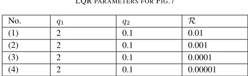
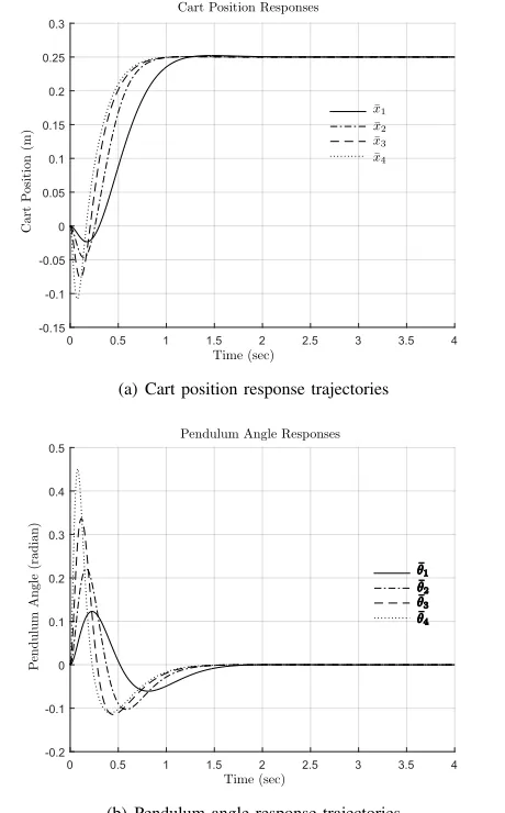
By adding the pregain, the steady state tracking error of the cart position is eliminated for all configuration in Table III in which the desired position of the cart is reached (r= 0.25m) (see Fig.7(a)). The transient time of the cart position response is improved slightly by reducing R. However, reducing R
also increases the overshoot of the pendulum angle response as shown in Fig.7(b). Furthermore, reducing R makes |Q|
relatively bigger thanR, the control system penalises the use of the control effortu. Referring to Table III and Fig.7(c), the
TABLE III LQRPARAMETERS FORFIG.7
No. q1 q2 R
(1) 2 0.1 0.01
(2) 2 0.1 0.001
(3) 2 0.1 0.0001
(4) 2 0.1 0.00001
required control input voltage is higher when R is smaller. For instance, the smallest R= 0.00001 requires the control input of115volts. In this configuration, the feedback gainK, the pregain, the characteristic polynomial function D(s) and its roots are found as follow
K = {−447.2,−333.5,−174.9−50.7}
¯
N = −447.21
D(s) = s4+ 60s3+ 1730s2
+13574s+ 35097 (63) s = {−24.8 + 24.2i,−24.8−24.2i,
−5.1 + 1.9i,−5.1−1.9i}
Further simulation experiments were conducted to fine tune the LQR parameters to obtain the fastest transient response where the controller input was contrained with the maximum value of 15 volts (half of the maximum voltage of the DC motor). The configurations used in these simulations are listed in Table IV. It can be seen on the Fig.8 that configuration (3)
TABLE IV LQRPARAMETERS FORFIG.8
No. q1 q2 R
(1) 2 0.1 0.01
(2) 2 0.01 0.01
(3) 4 0.1 0.01
(4) 4 0.5 0.00001
is the most satisfactory result which met the desired criteria. In this final configuration, the feedback gain K, the pregain, the characteristic polynomial function D(s) and its roots are found as follow
K = {−63.25,−69.54−30.83−10.91}
¯
N = −63.2456
D(s) = s4+ 31.2s3+ 434.2s2
+2364.4s+ 4963.5 (64) s = {−11.4 + 9.5i,−11.4−9.5i,
−4.2 + 2.2i,−4.2−2.2i}
V. CONCLUSIONS
0 0.5 1 1.5 2 2.5 3 3.5 4 -0.15
-0.1 -0.05 0 0.05 0.1 0.15 0.2 0.25 0.3
(a) Cart position response trajectories
0 0.5 1 1.5 2 2.5 3 3.5 4
-0.2 -0.1 0 0.1 0.2 0.3 0.4 0.5
(b) Pendulum angle response trajectories
0 0.5 1 1.5 2 2.5 3 3.5 4
-20 0 20 40 60 80 100 120
(c) Control ouput trajectories Fig. 7. State responses with pre-gain
involved state-feedback simulation after determining the con-trollability and observability of the system. It was assumed that the cart position x and the pendulum angle θ where available from sensor measurements. Hence, it was determined that by giving two sensor measurements was sufficient to construct a state-feedback system observable. Determining the gain matrix K was the important step in the optimal control
0 0.5 1 1.5
-0.1 -0.05 0 0.05 0.1 0.15 0.2 0.25 0.3
(a) Cart position response trajectories
0 0.5 1 1.5
-0.15 -0.1 -0.05 0 0.05 0.1 0.15 0.2 0.25 0.3
(b) Pendulum angle response trajectories
0 0.5 1 1.5
-5 0 5 10 15 20
(c) Control ouput trajectories Fig. 8. State responses with pre-gain
design. The optimality of the resulted gain matrix K was analysed by the performance cost functionJ. The parameters in the performance cost function, the LQR weightsQandR
by solving the Riccati Equation.
It is important to be noted that for the case of the tracking per-formance, where the controller effort should makey(t)≈r(t) as t→ ∞, hence the DC gain of the transfer function should be approximately 1. Therefore, it is necessary to scale the reference input using pregainN¯. Simulation experiments were systematically conducted by varying the configuration of Q
andR. Simulation results have been discussed in detail. The simulation results have shown that the larger Q and R the more you penalize the state and the control effort. Choosing a large value for R means that the controller stabilises the system with less (weighted) energy, it is called expensive control strategy. This control strategy is used when the control signal is constrained . On the contrary, choosing a small value for R means that the controller penalises the control signal (cheap control strategy), causing a large control signal. Large
Q implies less concern about the changes in the states.
ACKNOWLEDGMENT
Published results were acquired with the support of Min-istry of Research and Technology and Higher Education of Indonesia.
REFERENCES
[1] C. Wang, G. Yin, C. Liu, and W. Fu, “Design and simulation of inverted pendulum system based on the fractional pid controller,” in2016 IEEE 11th Conference on Industrial Electronics and Applications (ICIEA), June 2016, pp. 1760–1764.
[2] Z. Pengpeng, Z. Lei, and H. Yanhai, “Bp neural network control of single inverted pendulum,” inProceedings of 2013 3rd International Conference on Computer Science and Network Technology, Oct 2013, pp. 1259–1262. [3] M. H. Arbo, P. A. Raijmakers, and V. M. Mladenov, “Applications of neural networks for control of a double inverted pendulum,” in 12th Symposium on Neural Network Applications in Electrical Engineering (NEUREL), Nov 2014, pp. 89–92.
[4] G. O. Tirian, O. Prostean, I. Filip, and C. Rat, “Inverted pendulum controlled through fuzzy logic,” in2015 IEEE 10th Jubilee International Symposium on Applied Computational Intelligence and Informatics, May 2015, pp. 85–90.
[5] N. Metni, “Neuro-control of an inverted pendulum using genetic algo-rithm,” in2009 International Conference on Advances in Computational Tools for Engineering Applications, July 2009, pp. 27–33.
[6] R. F. Harrison, “Asymptotically optimal stabilising quadratic control of an inverted pendulum,”IEE Proceedings - Control Theory and Applications, vol. 150, no. 1, pp. 7–16, Jan 2003.
[7] D. Tabak, “Applications of mathematical programming techniques in optimal control: A survey,” IEEE Transactions on Automatic Control, vol. 15, no. 6, pp. 688–690, Dec 1970.
[8] P. Ignaciuk and A. Bartoszewicz, “Linear-quadratic optimal control of periodic-review perishable inventory systems,” IEEE Transactions on Control Systems Technology, vol. 20, no. 5, pp. 1400–1407, Sept 2012. [9] A. I. Bratcu, I. Munteanu, and E. Ceanga, “Optimal control of wind