Genetics and physical mapping studies on mouse chromosome 2

Genetic^and Physical Mapping Studies on Mouse

Chromosome 2

by

Stavros Males

A thesis submitted for the degree of

Doctor of Philosophy

at the

University of London

May 1995

The Galton Laboratory

ProQuest Number: 10018553

All rights reserved

INFORMATION TO ALL USERS

The quality of this reproduction is dependent upon the quality of the copy submitted.

In the unlikely event that the author did not send a complete manuscript and there are missing pages, these will be noted. Also, if material had to be removed,

a note will indicate the deletion.

uest.

ProQuest 10018553

Published by ProQuest LLC(2016). Copyright of the Dissertation is held by the Author.

All rights reserved.

This work is protected against unauthorized copying under Title 17, United States Code. Microform Edition © ProQuest LLC.

ProQuest LLC

789 East Eisenhower Parkway P.O. Box 1346

Abstract

This thesis describes two genetic maps of mouse chromosome 2 (MMU2), genetic maps relative to the wasted {wsf) and Ragged (Ra) mutations on distal MMU2 and a physical map of the region likely to contain the latter two genes.

The first two maps include 18 new PCR markers which were isolated from a subgenomic library constructed from a mouse-hamster somatic cell hybrid line whose main mouse-genome component was MMU2. Fourteen of these loci define microsatellite sequences and four represent randomly chosen DNA sequences. The maps were constructed using two interspecific backcrosses established using a laboratory mouse strain and mice from the related species Mus spretus. The inheritance pattern on MMU2 reveals loci that exhibit significant segregation distortion (SD) in males.

The genes responsible for the wasted (wsf) and ragged (Ra) phenotypes are very closely linked (0.2 cM) on the extreme end of MMU2. Two interspecific backcrosses segregating wst and Ra were set up in order to define the genetic position of these loci relative to currently available molecular markers. In total, 167 wstA/vst and 329 Ra/+ or +/+ mice were phenotyped for 5 microsatellites and two genes which, on the basis of the consensus map, would be expected to map near wst and Ra. The gene order established is;

D2Ucl1, Gnas- 1.8 cM + 1.0, D2Mit200- 1.8 cM + 1.0, D2Mit230 0.6 cM + 0.6, D2Mit74-0.6 cM + D2Mit74-0.6, Acra4- 0.6 cM + 0.6, D2Mit266, wst

D2Ucl1, Gnas- 1.2 cM + 0.6, D2Mit200- 0.6 cM + 0.4, D2Mit230- 0.6 cM + 0.4, D2Mit74, Acra4, D2Mit266, Ra

In an attempt to isolate flanking markers for both mutations, four overlapping yeast artificial chromosomes (YACs) were isolated and analysed by way of fluorescence in situ hybridisation (FISH), Southern blot and PCR analysis. These clones span a region of at least 360 kb and encompass the markers D2Mit74, Acra4 and D2Mit266\ the contig extends at least 200 kb proximal and 160 kb distal to Acra4. In the context of this work, a framework physical map extending 200 kb proximal and 310 kb distal to this gene was also established. Two YACs were found to span the T(2;16)28H translocation breakpoint. On the basis of these results, D2Mit74 is tentatively proposed to reside proximal to the breakpoint.

Table of contents

Title

Abstract

Dedication

Table of contents

List of figures

List of tables

Abbreviations Acknowledgments I II III IV IX XI XII XIV

Chapter 1 : Introduction

Part 1. Aims of the project

Part 2. The mouse in genetic analysis

2.1. Why mice

2.2. The establishment of inbred strains

2.2.1. Derivation of inbred strain

2.2.2. The development of congenic lines

2.3. Interspecific backcrosses

2.3.1. Uses of interspecific backcrosses 2.3.2. Limitations of interspecific backcrosses

Part 3. Molecular genetic analysis

3.1. The establishment of genetic maps

3.2. The discovery of DNA sequence variation

3.3. Microsatellites in genetic mapping

3.3.1. Structural features of microsatellites

3.3.2. Isolation and analysis of microsatellites sequences 3.3.3. Distribution of microsatellite sequences

3.3.4. Function of microsatellites 3.3.5. Uses of microsatellites

3.3.5.1. Tackling multifactorial diseases

3.4. Pathogenic microsatellites

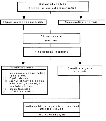
4.1. Positioning a mutant gene on the genetic and physical map 24

4.2. The isolation of molecular markers 26

4.2.1. Somatic cell hybrids 26

4.2.2. Chromosome microdissection 28

4.3. The story so far 29

Part 5. The wasted and ragged mouse mutants

31

5.1. The wasted mouse 31

5.1.1. Immunological abnormalities 31

5.1.2. Neurological abnormalities 34

5.2. The ragged mouse 36

Chapter 2: Materials and Methods

Part 1. General Techniques

39

1.1. Bacterial media, strains, antibiotics 39

1.1.1. Liquid and solid bacteriology media 39

1.1.2. Bacterial strains 39

1.1.3. Antibiotic stock solutions and working concentrations 39

1.2. Growth of bacterial cultures, storage media 39

1.2.1. Growth in liquid media 39

1.2.2. Growth on solid media 40

1.2.3. Preparation of competent cells 40

1.3. Propagation of bacteriophage X 40

1.3.1. Preparation of plate lysate stocks 40 1.3.2. Growth of bacteriophage X clones in a microtiter-format

arrangement 41

1.3.3. Storage of bacteriophage X lysates 41

1.4. Propagation of yeast cultures 41

1.4.1. Growth medium 41

1.4.2. Expansion of yeast cultures 41

1.4.2.1 Liquid cultures 42

1.4.2.2 Growth on solid media 42

1.4.3. Storage of yeast cultures 42

1.5. DNA extraction protocols 42

1.5.1. Extraction of total mouse/hamster genomic DNA 42 1.5.2. Extraction of total yeast DNA 43 1.5.3. Extraction of plasmid and bacteriophage X DNA 44 1.5.4. Immobilisation of high molecular weight DNA in agarose

blocks for PFGE 44

1.5.4.1. Mouse DNA 44

1.5.4 2. Yeast DNA 44

1.5.5. Quantification of DNA 45

1.6. DNA modification reactions 45

1.6.2. Déphosphorylation of DNA 46

1.6.3. Ligation of DNA 46

1.6.3.1. Subcloning of bacteriophage XDNA 47 1.6.31.1. Non-directional cloning 47 1.6.3.1.2. Directional cloning 47 16.3.1.3. Cloning of PCR products 47

1.7. Transformation of competent E.Coli cells 47

1.8. Immobilisation of colonies/plaques onto nylon membrane 48

1.8.1. Bacterial colonies 48

1.8.2. Bacteriophage X, plaques 48

1.8.3. Processing of membranes 48

1.9. In vlto DNA replication 49

1.9.1. Exponential amplification using the Polymerase Chain

Reaction 49

1.9.2. Radioactive labelling of DNA 49

1.9.3. DNA sequencing 50

1.10. Electrophoretic analysis of the DNA 51

1.10.1. Agarose gel electrophoresis of low molecular weight DNA 51 1.10.2. Pulse field gel electrophoresis (PFGE) of high molecular

weight DNA 52

1.10.3. Polyacrylamide gel electrophoresis 52 1.10.3.1. Non-denaturing polyacrylamide gels (native gels) 52 1.10.3.2. Denaturing polyacrylamide gels 53

1.11.Southern blotting 53

1.11.1. Salt transfer protocol 54

1.11.2. Alkaline DNA transfer 54

1.12. Hybridization of radlolabelled probes to Immobilised DNA 54

1.12.1. Hybridisation to plaque/colony DNA 55 1.12.2. Hybridisation to low and high molecular weight DNA 56

Part 2. The Isolation of molecular markers from mouse

chromosome 2

57

2.1. Construction of a subgenomic library from hybrid

line EBS-18/AZ 57

2.1.1. Partial fill-in, ligation and packaging reaction 59

2.2. Screening the mouse DNA-containIng clones for the presence

of (AC)n dinucleotlde repeats 60

2.3. Subcloning, cloning, screening and sequencing of the clones

with an (AC)n repeat 60

2.4. Genetic mapping of markers Isolated 61

2.4.1. The interspecific backcrosses and mapping of the markers

isolated 61

Part 3. Genetic and physical mapping near

wst

and

Ra

62

3.1. Genetic maps 62

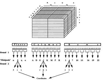
3.2. Screening of Yeast Artificial Chromosome (VAC) library 65 3.2.1. Screening of the library stacks 65 3.2.2. Screening individual stacks to determine the coordinates 65 3.2.3. Construction of vectorette libraries 67 3.2.3.1. Isolation of hybridisation probes by vectorette PCR 67 3.3 The mapping of the vitamin D 24-hydroxylase in the mouse 69 genome

Chapter 3: Results

Part 1 : The isolation of markers from MMU2

71

1.1. The isolation of mouse clones from hybrid line EBS-18/AZ 71

1.2. Screening for (AC)n microsatellites 73

1.3. Mapping 19 sequence tagged sites the mouse genome 75

1.3.1. Test for segregation distortion (SD) 82

Part 2: Genetic and physical maps near

wst

and

Ra

86

2.2. Genetic maps 86

2.2.1. Mapping Cyp24 in the mouse genome 88

2.3. Physical maps 90

2.3.1. The isolation of genomic clones from the Acra4 gene region 90 2.3.2. The isolation of yeast artificial chromosomes (YACs) 93 2.3.3. Molecular characterisation of four YACs 95 2.3.3.1. Fluorescence in situ hybridisation (FISH) analysis 98 2.3.3.2. Comparative analysis YACs using STSs and terminal 102 probes

2.4. The construction of a long range physical map either side of the

Acra4 gene region 111

2.4.1. PFGE analysis using probes proximal to Acra4 112 2.4.2. PFGE analysis using probes distal to Acra4 114

2.5. Overall conclusion from the physical mapping data 115

Chapter 4: Discussion

4.1. The isolation and mapping of 19 STSs in the mouse genome 118 4.1.1. D__Ucl markers mapping close to mouse mutations 119 4.1.2. Evidence of segregation distortion 119 4.2. Genetic and physical maps near wasted (wsf) and ragged (Ra) 121

4.2.1. Genetic maps 121

4.2.1.1. Prospects for positioning Ra and wst on the genetic map 122

4.2.2. The physical map 123

4.3. Candidate genes fo r wst and Ra 125

4.3.1. Wasted 125

4.3.2. Ragged 128

4.5. What needs to be done 129

Appendix

The phenotypes of mice segregating Ra and wst 131 Complete DNA sequences of all clones sequenced from LibEBSISAZ 144

Bibliography

1

S

2

List of Figures

1.1. A consensus linkage map of mouse Chromosome 2 2 1.2. Pedigree analysis of a 147-animal, N2 progeny, generated by an

interspecific backcross and localisation of a new molecular marker X 11

1.3. Stuctural features of a microsatellite sequence 15 1.4. A schematic outline of the steps involved in positional cloning 25 2.1. A composite linkage and cytogenetic map of mouse chromosome 2 showing

the position of the markers present in the hybrid cell line EBS-18/AZ 58 2.2. Lambda GEM-11 Xho I half-site arms cloning strategy 59 2.3. Schematic outline of the screening of the two mouse YAC libraries 66 2.4. Schematic outline of the vectorette PCR approach 68 3.1. The result from the screening of two plates from library

LibEBS18AZ with radiolabelled mouse DNA 71 3.2. A duplicated array of mouse DNA-containing bacteriophage X clones

hybridised to a (GT)is oligonucleotide 74

3.3. Haplotype analysis of 94 N2 progeny from the BSB and BSS

backcrosses for MMU2 markers 78

3.4. Linkage map of mouse chromosomes 2 (MMU2) and 7 (MMU7)

showing the position of the D_Ucl markers 80

3.5. Examples of electrophoretic analysis used to establish the phenotypes

at three D_Ucl loci. 81

3.6. Graphic representation of the proportion (P) of heterozygous males,

females and total number of BSB/BSS backcross progeny 83 3.7. Pedigree analysis of N2 offspring derived from the ragged and

wasted backcrosses 87

3.8. Linkage maps of distal MMU2 near wst and Ra loci derived from the data

shown in figure 3.7 87

3.9. Linkage map of distal MMU2 showing the position of Cyp24 89 3.10. Silver-stained polyacrylamide gel used to establish the phenotypes

at Cyp24 of the N2 progeny in the ragged backcross 89 3.11. Partial physical map of a 9 kilobase region derived from clone CD A4 91 3.12. Phenotypes of critical recombinant mice across clone CDA4 92 3.13. The screening of the two YAC libraries for the Acra4 region 94 3.14. Pulse field gel electrophoresis and Southern blot analysis of the 4

YACs to determine their size and stability 95

3.16. Cytogenetic maps of MMU2, MMU8 and MMU16 showing the position of the breakpoints associated with the translocations T(2;8)2Wa or

T2Wa and T(2;16)28H or T28H 98

3.17. Fluorescence in situ hybridisation analysis of YACs ICRF8, ICRF21 and

SM2 99

3.18. PCR analysis of YACs ICRF8/21 and SM2/21 for the presence of three

STSs 103

3.19. PCR analysis of the 4 YACs for the presence of D2Mit266 and the two

terminal STSs from clone SM29 104

3.20. Southern blot analysis of clone ICRF/8/21 and SM2 106 3.21. The hybridisation pattern for terminal probe ICRF21-1 107 3.22. A YAC contig encompassing markers D2Mit266, Acra4 and D2Mit74 108 3.23. Long range physical map near the Acra4 gene region 111 3.24. PFGE and Southern blot analysis using probes proximal to the Acra4 112

gene region

List of Tables

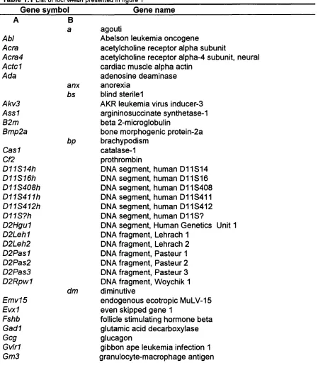
1.1. List of loci which presented in figure 1 3

1.2. A summary of cytokine expression in wasted mice 32 2.1. Details of the markers mapped relative to ragged and wasted 64

3.1. The results from the screening of library LibEBSISAZ to isolate mouse

clones 71

3.2. Results from screening the mouse clones for the presence of (AC)n

microsatellites 73

3.3. Details of the microsatellites and other Sequence Tagged Sites (STS)

mapped in the mouse genome 76

3.4. Chi-Square analysis of the total number of Mus spretus and C57BL/6J

alelles in the BSB and BSS backcrosses 84

3.5. Chi-square analysis of the number of Mus spretus and C57BL/6J

allele based on the recombinant chromosomal haplotypes of the BSB and

BSS backcrosses 85

3.6. PCR primer sequences and PCR product sizes in clone CDA4 91

Abbreviations

bp base pairs

BSA bovine serum albumin cDNA complementary DNA

Ci Curie

CIP calf intestinal phosphatase cM centiMorgan

cm centimetre

dATP 2’-deoxyadenosine 5’-triphosphate dCTP 2’-deoxycytosine 5'-triphosphate ddH20 deionised and distilled water dGTP 2’-deoxyguanine 5'-triphosphate DNA 2'-deoxyribonucleic acid

dNTP deoxynucleotide triphosphate dTTP 2’-deoxythymidine 5'-triphosphate DTT Dithiothreitol

EDTA Ethylenediaminetetra-acetic acid E.coli Escherichia coli

FISH Fluoresence in situ hybridisation

g grams

g acceleration due to gravity (9.8 ms'^) HSA20 human chromosome 20

HMW high molecular weight kb kilobase pair

M Molar

mM millimolar Mb Megabase mg milligram ml millilitre pi microlitre pg microgram ng nanogram

nAchR nicotinic acetylcholine receptor PCR polymerase Chain Reaction PFGE pulse-field gel electrophoresis

SSC saline sodium citrate

SSCA single strand conformation analysis STS sequence tagged site

Tris tris hydroxymethyl aminomethane

u units

UV ultra violet

% volume for volume ^/v weight for volume

Acknowledgments

I am particularly thankful to Dr Cathy Abbott who has devoted so much time and effort supervising this work. I hope Tom will forgive me for occupying some of his mother’s time. I am greatly indebted to Prof. Sue Povey for her advice, understanding and help during the latter part of this work. A special thank you to Dr Dennis Stephenson for his advice while preparing this thesis.

I am grateful to the Wellcome Trust which supported this work. Successive heads of the Galton Laboratory namely Professors Elizabeth Robson and Steve Jones and Dr Jonathan Wolfe have been very generous in contributing towards the cost of this project and I thank them for their commitment. I thank Alison for helping me to get this project to a fine start and both Alison and Lorna for sharing some of their data with me. I fear chocolate-cake and cappuccino consumption will stay with Lorna for some time. Special thanks to Dr Jo Peters and Simon Ball for managing the backcrosses at the MRC Radiobiology Unit (HanA/ell) and Liz Dutton and Dr Margaret Fox for the FISH analysis.

CHAPTER 1 : INTRODUCTION

Part 1 : Aims of the Project

This project was initiated in October 1991 with two main objectives. First, to generate a set of molecular genetic markers for mouse chromosome 2 (MMU2). Second, to construct a genetic and, depending on the density of that map, a physical map of the region containing the genes responsible for the wasted (wst) and ragged (Ra) mouse mutants; greater emphasis was placed towards isolating the region which harbours wst.

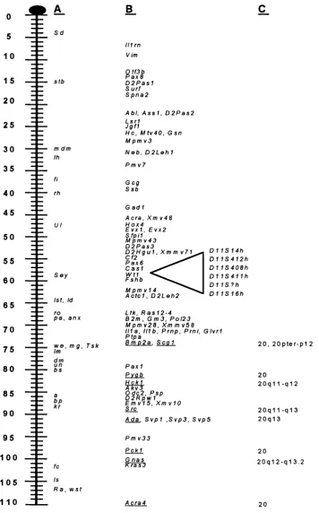
When this work begun, the consensus genetic linkage map of MMU2 consisted of 80 molecular markers and twenty nine genes responsible for developmental mutations (figl.1; table 1.1). At this marker density (on average 1 marker every 1.4 cM), it would be very difficult to isolate any of these mutations by way of positional cloning or construct a high resolution genetic map of MMU2, unless more markers became available. This study was therefore initiated to generate additional molecular markers for this chromosome. Microsatellites were considered to be the most useful loci for genetic analysis (Weber and May, 1989), so such sequences were specifically targeted for isolation. The DNA source was a mouse- hamster somatic cell hybrid line containing the whole of mouse chromosome 2, the proximal domain of mouse chromosome 15 and possibly submicroscopic fragments of other mouse chromosomes (Peter Lalley, personal communication). The strategy was to construct a subgenomic library from this hybrid cell line and screen it with a composite probe, derived by radiolabelling total mouse DNA, in order to isolate mouse-DNA containing clones. It was anticipated that the majority of the clones isolated would originate from MMU2, as it was the major mouse-genome component in this cell line. Two interspecific backcrosses, established at the Jackson Laboratory, were used to map the markers produced in this way.

Figure 1.1 A consensus linkage map of mouse Chromosome 2. The loci listed in column A represent 27 genes responsible for developmental mutations. Two genes, namely those for curly-tail lethal (Cyl) and fathead (fhd) do not appear on this map, as th ^h a v e only been mapped in two point crosses and their position on the map relative to other markers is not known. Column B lists the loci for which molecular probes are available. The genes whose homologues have been mapped to HSA 20 are underlined and the respective region is shown in column C (derived from Siracusa and Abbott, 1991; Pilz et al., 1992).

G 5 1 G

1 5 2G 2 5 3G 3 5 4G 4 5 5G 5 5 6G 6 5 7G 7 5 8G 8 5 9G 9 5 1 GG

1 G5 1 1 G

B

S d

st b

m dm Ih

fi rh

Ul

S e y

1st, Id ro p a , a n x

w e , m g, T s k Im dm un bs a fc Is R a , w s t

111 rn Vi m

Ot f Sb P a x B D 2 P a s 1 S ur f S p n a 2

Abl , A s s 1, D 2 P a s 2

jVfl

H c , M t v 4 0 , G sn M p m v3

N e b, D 2 L e h 1 P m v 7

G cg S sb

G a d i A er a, X m v 4 8 H o x 4 E v x l , E v x 2

W p mv 4 3 D 2 P a s 3

D 2 H g u 1 , X m m v 7 1 C f 2

P a x 6 C a s i

ÏÏJL

M p m v 1 4 A c t c l , D 2 L e h 2

D 1 1 S 1 4 h D 1 1 S 4 1 2 h D 1 1 S 4 0 8 h D 1 1 S 4 1 1 h D 1 1 S ? h D 1 1 S 1 6 h

Lt k, R a s 1 2 - 4 B 2 m , G m 3 , P o l 2 3 M pm v 2 8 , X m m v 5 8 I l i a , 111b, P r n p , Pr ni , G I v r I P t p a

Bm o 2 a . S e a l

P a x 1 P v Qb

E m v l 5, X m v i o Sr e

A da. S v p l , S v p 3 , S v p 5

P m v 3 3 P e k l G n a s k r a s 3

A er a 4

2 0 , 2 0 p t e r - p 1 2

20

2 0 q 1 1 - q1 2

2 0 q 1 1 - q1 3 2 0 q 1 3

20

2 0 q 1 2 - q 1 3 . 2

Genes mapping to human chromosome 20 (HSA 20) appear to be confined to the distal domain of mouse chromosome 2 (figure 1.1). While the localisation of these genes to HSA 20 is based upon physical mapping studies (Grzeschik and Skolnick, 1991), the data for MMU2 is based exclusively on genetic linkage studies. Nevertheless, the order of genes appears to be conserved in the two species. Given the observation that the consensus map placed wst and Ra in a conserved region with 20q13.2-qter, it seemed reasonable to establish whether genes mapping to this region of the human genome mapped in close proximity to these two mutant genes.

Table 1.1 List of loci w N d i presented in figure 1

Gene symbol Gene name

Abl Acra Acra4 A c td Ada Akv3 Ass1 B2m Bmp2a Cas1 Cf2 D11S14h D11S16h D11S408h D11S411h D11S412h D11S?h D2Hgu1 D2Leh1 D2Leh2 D2Pas1 D2Pas2 D2Pas3 D2Rpw1 Emv15 Evx1 Fshb Gad1 Gcg Gvlr1 Gm3 B a anx bs bp dm agouti

Abelson leukemia oncogene

acetylcholine receptor alpha subunit

acetylcholine receptor alpha-4 subunit, neural cardiac muscle alpha actin

adenosine deaminase anorexia

blind sterile 1

AKR leukemia virus inducer-3 argininosuccinate synthetase-1 beta 2-microglobulin

bone morphogenic protein-2a brachypodism

catalase-1 prothrombin

DNA segment, human D11S14 DNA segment, human D11S16 DNA segment, human D11S408 DNA segment, human D11S411 DNA segment, human D11S412 DNA segment, human D11S?

DNA segment. Human Genetics Unit 1 DNA fragment, Lehrach 1

DNA fragment, Lehrach 2 DNA fragment, Pasteur 1 DNA fragment, Pasteur 2 DNA fragment, Pasteur 3 DNA fragment, Woychik 1 diminutive

endogenous ecotropic MuLV-15 even skipped gene 1

follicle stimulating hormone beta glutamic acid decarboxylase glucagon

Table 1.1 continued

Gnas Gs protein alpha, stimulatory regulator

Gsn gelsolin

Hc Hemolytic complement component 5 Hck1 hematopoietic cell kinase 1

H 0x4 homeo box-d gene cluster

Hsp842 heat shock protein 84 kDa2

111a interleukin 1 alpha 111b interleukin 2 beta

Hlm interleukin 1 receptor antagonist

J g fi anonymous mouse cDNA

kr kreisler

Kras3 Kirsten rat sarcoma oncogene 3

Id limb deformity Ih lethargic Im lethal milk Is lethal spotting 1st Strong’s luxoid

Ltk leukocyte tyrosine kinase

mdm muscular dystrophy with myositis mg mahogany

Mpmv3 modified polytropic MuLV provirus 3

Mpmv14 modified polytropic MuLV provirus 14 Mpmv28 modified polytropic MuLV provirus 28 Mpmv43 modified polytropic MuLV provirus 43

Mtv40 mouse mammary tumour virus 30

Neb nebulin

Odc2 ornithine decarboxylase 2

Otf3b octamer transcription factor

pa pallid

P axi paired box 1

Pax6 paired box 6

Pax8 paired box 8

P ckl phosphoenolpyruvate carboxylase 1

Pmv7 polytropic murine virus 7

Pmv33 polytropic murine virus 33

Pol23 viral polymerase

Psp parotid secretory protein

Ptpa receptor tyrosine phospatase alpha Pygb brain glycogen phosphorylase

Ra ragged

Ras12-4 ras-like gene12-4

Rec2 ecotropic MuLV M813 receptor rh rachiterata

ro rough

S cgi secretogranin 1 (chromogranin B) Sd Danforth’s short tail

Sey small eye

S fpil SFFV proviral integration 1

Sgnel neuroendocrine protein 7B2

Spna2 alpha spectrin 2, brain

Spna2 alpha spectrin 2, brain

Src Rous sarcoma oncogene

Table 1.1 continued

stb stubby

Surf surfeit gene cluster Svp1 seminal vesicle protein 1 Svp2 seminal vesicle protein 2 Svp5 seminal vesicle protein 5

Tsk tight skin

Ul ulnaless

an undulated

Vim vimentin

we wellhaarig wst wasted

W tl Wilms tumour homolog

Xmmv58 xenotropic MCF leukemia virus 58

Xmmv71 xenotropic MCF leukemia virus 71

XmvW xenotropic murine leukemia virus 10

Xmv48 xenotropic murine leukemia virus 48

Part 2: The Mouse in Genetic Analysis

2.1 Why mice

The mouse was chosen as the principal experimental animal to help unravel the structure and function of the coding component of the human genome. The human genome project (HGP) was primarily initiated to improve public health by analysing the causes of inherited diseases (McKusick and Amberger, 1994) and develop preventative and therapeutic treatment for these conditions. The goal of the HGP is the provision of detailed genetic and physical maps for all chromosomes, as a prelude to the determination of the complete DNA sequence of the human (Cox et al., 1994).

The haploid gene content of the mouse and human genomes is thought to be very similar, approximately 80,000 genes (Antequera and Bird, 1993), although more conservative estimates have also been proposed (Fields at a!., 1994). Experience has shown that the majority of human genes have homologous sequences in the mouse genome (Copeland at a!., 1993). It is not clear how many of our genes have homologous (or orthoiogous) counterparts in the mouse genome, but the number of human genes with no mouse homologues will probably be very small. More importantly, as the genetic position of homologous DNA sequences is being determined in both species, it becomes apparent that many genes have retained their physical association in conserved linkage groups (Nadeau, 1989; O’Brien at a/., 1993; Copeland at a!., 1993). The extensive comparative maps now available provide an efficient way to predict the position of new genes on the human map by mapping them in the mouse. Conversely, the position of genes in the mouse genome can be predicted from mapping information in humans (e.g. Malas at a!., 1994). The expansion of the comparative map will primarily progress through genetic mapping, although some data from physical mapping will be necessary as the density of the map increases. In the mouse, genetic mapping is very powerful and very simple (see below). Hundreds or even thousands of genes can be mapped in multipoint crosses and the mapping information should be directly relevant to the human genome mapping effort (Copeland at a!., 1993). Strategies are now being initiated to maximise the efficiency and efficacy of the HGP by isolating and cataloguing all the genes in humans and mice. This represents a more efficient use of limited resources than the often more redundant effort to identify individual genes during existing research programs (Chapman at a!., 1993).

underscore the similarities and differences in the process of development between mice and humans and lend credence to efforts attempting to reproduce human pathological conditions by manipulating the mouse genome (reviewed by Yamamura and Wakasugi, 1991; Gossen and Vijg, 1993; Gatherer, 1993; Davidson et al., 1995). The advances in transgenic technology have been used to induce human disorders by introducing defective human genes in mice (Stacey at a!., 1988). Similarly, endogenous mouse genes can be specifically disrupted in pluripotent embryonic stem (ES) cells, which can be selected and reintroduced back into a developing embryo (Capecchi, 1989; Rossant and Joyner, 1989; Davidson at a/., 1995). The advances in gene technology will enable attempts to treat human diseases by somatic-gene therapy protocols. The mouse is an excellent model organism to advance these techniques and test their potential for intervening in order to correct defects in our code (Porteous and Dorin, 1993; Friedmann, 1994).

The choice of the mouse is also based on many practical considerations. Mice are easy to handle and cheap to maintain. They reach sexual maturity six weeks after birth. An average breeding female has between four to eight litters and the gestation period is between nineteen and twenty days. Each litter contains six to eight pups (Hogan, 1986). Thus, crosses can be set up at will to generate a very large number of progeny in a relatively short period of time. The temporal and spatial pattern of expression of genes can be readily studied, for the use of mice allows access to all tissues at every stage of development.

2.2 The establishment of inbred strains

A genetic map is the most important tool of a geneticist. The development of the mouse linkage map would not have progressed at the pace that it has done (Silver at a!., 1994), had genetically homogenous strains not been available. Mice have been studied since the turn of the century, mainly in the quest for cancer treatment. The first attempts to treat cancers in mice led to puzzling observations; the response to the treatment was different even between animals from the same litter. It was thought that genetic heterogeneity was to “blame” for these differences and breeding strategies were devised to “eliminate” it.

inheritance (Resting, 1979 and references therein). The first set of inbred strains, established just after the end of World War II, led to the identification of these genes that are now known to code for the histocompatibilty antigens (Snell, 1981; Lindahl, 1991).

2.2.1 Derivation of inbred strains

Inbred strains are derived by continuous full brother x sister (known as full- sib) matings, or by parent-offspring mating. Genetically, both types of matings are equivalent. A strain is regarded as inbred after twenty consecutive generations of full-sib matings (Staats, 1968 and 1976). In the case of parent-offspring matings this rule also applies, provided the mating in each case is to the younger of the two parents. In the twentieth generation the members of an inbred strain should trace back to a single ancestral pair. All mice of this generation will be homozygous at virtually all loci and all progeny subsequently produced will be genetically identical or isogenic, barring residual segregation or mutation. Isogenicity is the correct genetic description attribute of the members of an inbred strain. The term “inbred” describes a breeding method rather than a genetic property but its wide use has come to mean the latter. The colonies of inbred strains are maintained by continued brother sister mating so that the occurrence of new mutations can be quickly detected.

Laboratory lines are thought to originate from two subspecies of the complex species Mus musculus, namely Mus musculus musculus and Mus musculus domesticus (reviewed by Bonhomme and Guenet ,1989). However, certain allelic variants observed in inbred lines have not been observed in either of these two subspecies and it was proposed that multiple mouse species might have contributed to the derivation of experimental mouse lines (Blank et al., 1986). Included in the Mus musculus species are the subspecies Mus musculus castaneus and Mus musculus bactrianus. All four groups breed in the wild to produce fertile hybrids (Moriwaki at a/., 1986). Three additional species of the genus Mus are found in Europe, namely Mus spicilegus, Mus spretus and Mus 4A.. Mus spretus shows the greatest degree of allelic variation among these species (Bonhomme et al., 1984) and has been of enormous value in segregation analysis in recent years (see below).

2.2.2 The development of congenic lines

can be developed by either twenty generations of full-sib matings with forced selection for a desired locus (hereafter referred to as “control locus”) or by seven to twelve generations of backcrossing to an established inbred strain (Klein, 1975). For the backcross system the animals in each generation receive half of their entire genome from the inbred strain. Hence theoretically, the genes that came in with the control locus and are not linked to it will be replaced by those contributed by the inbred strain at a rate of 50% in each generation. In consecutive generations, the proportion of these loci will diminish by 1-1/2-1/4-1/8-1/16 and so on, or 1-(1/2)"'\ After seven generations, the probability of homozygosity for an allele of the inbred strain is 98.4% { 1-(1/2)®} which increases to only 99.9% after twelve generations of backcrossing. In the case of loci which are linked to the control locus, the chance of homozygosity is 1 - (1-c)"'^ (c defines the estimated recombination frequency between the control locus and any locus associated with it). After twelve generations, the probability of homozygosity at a locus 10 cM (c=0.1) away from the control one is 68.6%. The region that harbours the control locus, known as the passenger region, diminishes in length in advancing generations and bears the control locus plus a few other closely linked DNA segments.

This particular property of congenic lines was exploited in attempts to isolate developmental mutations. Two different approaches are briefly outlined. Rikke and his colleagues (1993) attempted to isolate markers near the pearl locus. Pearl is an autosomal recessive mutation causing hypopigmentation of the coat and the eyes (Sarvella, 1954). It arose on a C3H stock and was transferred to a C57BL76J background (Sarvella, 1954). A congenic hybrid line was generated which carried the wild type allele from Mus spretus, on a Mus musculus domesticus background by repeated backcrossing for twelve generations, followed by an additional twelve generations of full-sib matings (Rikke et a/., 1993). A genomic library was then constructed from this line and screened with LINE-1 oligonucleotides, (LINE-1 is a member of the long interspersed repeats, reviewed in Hastie, 1989), which specifically detected clones of Mus spretus origin (Rikke et a!., 1991; Rikke and Hardies, 1991). Some of the positive clones that were tested were shown to be linked to the pearl locus as expected (Rikke et a/., 1993).

was thought to be closely linked to Ebfj4.2 based on the consensus linkage map (White et al., 1992). The restriction fragment length pattern from C57BL/6J mice and pallid congenic mice at the Ebp4.2 locus was different, providing evidence of the proximity between pa and Ehp4.2 without the need to set up a cross and map pa relative to Ebp42 . Ebp42 was proposed to be allelic to pa due to the presence of an aberrant mRNA species in affected tissues (White et al., 1992).

Notwithstanding some elegant features associated with congenic lines, their use in the ways just described would probably remained very limited. This is because their development requires many generations of breeding which can take up to years before any analysis can be performed. Only the lines that already exist could conceivably be used for such experiments. As the density of the mouse genetic map advances at a galloping pace, many markers are likely to co-localise with genes responsible for phenotypic deviants on the consensus genetic map. If well- characterised congenic lines are available for such loci, it should be possible to identify the markers closely linked to an individual control locus by determining the phenotype of the congenic and parent strains. The markers with a phenotype unique to a congenic line, assumed to originate from alleles from the donor strain, should theoretically be the ones to choose for multilocus segregation analysis, thus reducing the effort of having to map every marker likely to be linked to the control locus.

Studies using congenic lines have demonstrated the effect of the genetic background on the presentation of a genetically determined trait. For example, the recessive mutation dystrophia musculahs has two allelic variants, dy and , which arose on the strains 129/Re and WK/Re respectively (Green, 1989). Homozygotes of the type have a milder phenotype than dy/dy ones when studied on WK/Re background but a similar clinical and histological profile when studied on 129/RE background (MacPike and Meier, 1976). Keeping the genetic background the same in different congenic lines allows a more detailed study of the effects that are intrinsically associated with a mutation. For example, the relationship between the major histocompatibility complex and life-span in mice was studied by Smith and Walford (1977). Several lines with various H-2 haplotypes were maintained on an identical inbred parent line. Very significant differences in life-span were noted between lines bred on the same genetic background, suggesting that the H-2 complex has important effect on life-span (Smith and Walford, 1977).

2.3 Interspecific backcrosses.

genetic material between homologous chromosomes during meiosis to be detected. It is also important to be able to map as many loci as possible on a single cross and generate a comprehensive linkage map.

The introduction of interspecific crosses sparked off an explosion in mouse genetic mapping. Mus spretus is one of the most distantly related Mus species that interbreeds with laboratory mice to produce fertile F1 females (Avner, 1988), the FI males being sterile (Matsuda et al., 1991). Because of the inherent genetic diversity between the two progenitor species, the FI parents are likely to be heterozygous at practically every locus. DNA sequence differences identified in the form of restriction fragment length variants, RFLVs (Botstein at a/., 1980), can be easily identified using only a very limited number of restriction endonucleases. FI interspecific female hybrids can be backcrossed to either species to generate an N2 segregating progeny. In order to build up a genetic map, the progeny is first phenotyped for a series of evenly spaced markers whose order on a chromosome is not in dispute, to serve as anchors for placing new markers on the map. Most recombination events can be deduced through this preliminary set of phenotypes. As more markers are placed on each chromosome, all the recombination events are deduced and the chromosomal haplotypes of each progeny member is being determined. A new locus can then be assigned precisely on a chromosome by analysing its segregation in the progeny and placing it at a position that will minimise the number of double or multiple recombination events. This exercise is called ‘pedigree analysis’ and is illustrated in figure 1.2.

Figure 1.2 Pedigree analysis of a 147-animal, N2 progeny, generated by an interspecific backcross and localisation of a new molecular marker X. Each vertical array of boxes represents a different chromosomal haplotype. The filled squares denote the laboratory-mouse alleles and the open squares the Mus spretus alleles. The animals have been phenotyped for ten markers, a to j, on a single chromosome. All animals share an identical chromosome derived from one of the backcross parents. The numbers at the bottom indicate the number of animals that share a particular haplotype. These numbers change as new markers are added to the map, and new haplotypes are deduced. The two haplotypes (patterned arrows) help localise marker X between markers c and d. This is the only position on the map that will not generate any double recombination events (modified from Avner, 1988).

B a c k c r o s s h a p l o t y p e s

C E N *

□ □ m C2mc2 m a m □

--- ►

m a m a m a m a m

□ a a m o m a m □ m a m a m a m a □ a m a a m a m □ m a m a m a m a □ a m a m a a m □ ■ 1=1 ■ o ■ □ ■ o

□ ■ ( = ! ■ □ ■ o

□ a m a m a m a □ □ m a m a m a □ a m a m a m a a m a a m a m a □ a m a m a m a a m □ ■ [=11=1 ■ o ■ □ a m a m a m a 1=1 ■ 1=1 ■ l = I O

□ a m a m a m a a m a m a m a m 1=1

43 50 8 6 4 1 3 5 2 1 0 1 2 2 1 1 5 8 1 3

P h e n o t y p e s

Pedigree analysis takes into account the phenomenon of genetic interference which was first introduced by Morgan and his colleagues to explain the genetic data that were obtained from Drosophila crosses. Interference is the tendency of an already established chiasma to suppress the formation of other chiasmata in the nearby region. This phenomenon is also thought to occur in mice, the evidence being the apparent paucity of double/multiple crossover events detected on chromosomes from segregating progenies (Blank et ai, 1988; Justice and Bode, 1988). There is no cut-off value of recombination frequency or physical distance beyond which double recombinants are permitted; instead the number of double recombination events between markers is kept to the minimum as the genetic distance decreases. As more physical data become available, it should be possible to determine whether interference diminishes as a function of genetic or physical distance (Foss et a!., 1993).

2.3.1 Uses of interspecific backcrosses.

Comparative mapping through interspecific or intrasubspecific crosses offers an unparalleled resource for mapping loci whose order cannot be resolved in humans through family studies. Many genes in humans are assigned to individual chromosomes by fluorescence in situ hybridisation, as it is a very quick way for gene localisation. The mapping of these genes on the genetic map is the next priority, and the use of mouse crosses to construct genetic maps is a more efficient and cost effective approach, provided human complementary DNA (cDNA) probes are available and detect the mouse homologous gene sequences. Their tentative position on the human map could then be predicted based on the comparative map.

Several investigations have reported that in interspecific backcrosses, the transmission ratio of 1:1, expected in a diallelic system, is significantly distorted in favour of one of the parental alleles (e.g. Copeland e t a!., 1993; Siracusa e t al.,

1991; Rowe e t al., 1994;). This phenomeno/iis called segregation distortion (SO) and sex-specific differences in allelic inheritance for certain chromosomal regions on MMU2 have been reported (Siracusa et a!., 1991; this study). The factors likely to drive SD remain unclear, but they are likely to be due^cfifferential embryonic survival through the action of different allelic combinations or the action of individual alleles. The mapping and cloning of these loci seems possible, if haplotypes that favour distortion are backcrossed to either of the progenitor species (Siracusa e t al., 1991). SD will be further discussed in the light of the data presented in this study.

2 .3 .2 Lim itations of in te rs p ecific b ackcrosses

The linkage maps derived from interspecific crosses are derived from data from female meiotic recombination. Therefore, linkage information for the X-Y pseudoautosomal region cannot be obtained. The use of M as musculus castan eu s

or M us musculus molossinus as the wild mouse parent can overcome this problem

(e.g. Buckwalter e t al., 1991). These are subspecies of the M us m usculus species that exhibit very high degree of genetic divergence from laboratory lines and both sexes in the FI progeny are fertile (Guenet, 1986). So far, there appear to be no gross differences in the organisation of the M us spretus genome, compared to that of the laboratory mouse, apart from a small inversion in the proximal region of chromosome 17 (Hammer e t al., 1989). Areas which display very significant

Part 3: Molecular Genetic Analysis

3.1 The establishment of genetic maps

Fifteen years ago, the idea of constructing a genetic map of the mouse and human genomes was a distant dream. The major barrier to genetic analysis was the lack of suitable polymorphic® mendelian markers. Even with experimental mammalian species, such as the mouse where a large number of morphological variants had been collected (Silvers, 1979; Green, 1989) and optimum matings could be imposed, it was not possible to construct complete maps. The dream of a complete map only became possible when it was realised that variation found at the DNA sequence level could be exploited as genetic markers (Botstein et al., 1980). The long-established classical genetics found the perfect match - molecular genetics.

3.2 The discovery of DNA sequence variation

The p-globin locus was the first to have been studied systematically in normal individuals (Jeffreys, 1979). Sequence variants were assayed by the gain or loss of a restriction enzyme site and found to be present every few hundred base pairs. These variants could be resolved on Southern blots (Southern, 1975) and it was quickly realised that they could be used for map construction because they were potentially unlimited and polymorphic (Botstein, 1980). Restriction fragment length polymorphisms (RFLPs) transformed human genetics. For the first time, maps for the whole genome could be constructed and the mapping of genes causing diseases with Mendelian inheritance became an achievable goal. However, RFLPs are not ideal for creating maps. An ideal marker should be highly polymorphic and exist in many different alleles, thus maximising the chance of the parents being heterozygous and enabling the identification of allelic variants across generations. The vast majority of RFLPs are caused by the loss or gain of a restriction enzyme site and have only two forms. The second drawback is that the analysis of RFLPs requires significant amounts of DNA and the technology involved is less amenable to automation than other systems. For mouse genome mapping restriction fragment length variation (RFLV) analysis is the principal method for mapping genes isolated from distant species such as humans, as the polymerase chain reaction (PCR; Saiki et a!., 1988) is not always applicable.

3.3 Microsatellites in Genetic Mapping

Two discoveries have revolutionised current genetic mapping strategies in mice. The introduction of interspecific and intersubspecific backcrosses and the realisation that an abundant class of simple sequence repeats, known as microsatellites (Hamada et a!., 1982), displays high levels of allelic variation both in

humans and mice (Weber and May, 1989; Tautz, 1989; Litt and Luty, 1989; Smeets et al., 1989; Love et al., 1990; Hearne et al., 1991; Cornall et al., 1991; McAleer et al., 1992). Fortunately for mouse geneticists, the arduous task to identify most of the microsatellites known today was undertaken by only one research group who isolated and mapped more than four thousand of such loci (Dietrich et al., 1992 and 1994). By the end of 1995 this number will rise to 6000 and this will perhaps be one of the most remarkable achievements in mouse genetics this century.

3.3.1 S tru c tu ra l Features of M icrosatellite Sequences

The basic structure of a microsatellite is depicted in figure 1.3. This consists of an array of mono-, di, tri- or tetranucleotides arranged in tandem. Microsatellites are also called simple sequence repeats (SSRs).

Figure 1.3 Stuctural features of a microsatellite sequence. A polymorphic SSR containing a variabie number of core repeats (filled boxes) flanked by the same single copy DNA sequence.

G AT CTT CG AT CCTT G G AT C G T ACT G G CT AG CT AAT G C

G A T C T T C G A T C C T T G G A T C ^ ^ ^ 'X : V i V . : T : ' l ': ' J « j i G T A C T G G C T A G C T A A T G C G A T C T T C G A T C C T T G G A T C ^ iiæ s ijM :::fc :^ --j;ÿ v J ^ t^ s a n T A r T G G r : T A G r T A A T G r :

G AT CT T CG AT CCT T G G AT C G T A C T G G C T A G C T AAT G C

G A T C T T C G A T C C T T G G A T C G T ACT G G CT AG CT AAT G C

GATCTTCGATCCTTGGATCrr^.'fT^^^^^^^

G A T C T T C G A T C C T T G G A T C m C K # . % . : ; i i . .; T : j : ^ n i ^ G T A C T G G C T A G C T A A T G C

G AT C TT CG AT CC TT G G A TC t f G T AGTGG C.T AG CT AAT G C.

Occasionally, the repeat array is interrupted by the insertion of other nucleotides (usually mono- or dinucleotides) to form an imperfect repeat. Other microsatellites consists of two or more different runs of repeats and are classified as compound. By far the most extensively studied class of microsatellites is of the (AC)n

type and the information given below refers to this type unless stated otherwise. In humans, the level of variation appears to increase as the number of repeats increases (Weber, 1990). Sequences with roughly twelve or more repeats are more likely to be polymorphic than shorter sequences and have PIC^ values greater than 0.7. Imperfect repeats show a relatively low level of allelic variation irrespective of their length (Weber, 1990). In the mouse, the microsatellite variation among laboratory strains is about 50% on average; between laboratory strains and the subspecies Mus musculus castaneus or the separate species Mus spretus, it is over 90% (Dietrich et ai, 1994).

When microsatellites were first studied in a prokaryotic system, it was

W ---Polymorphic Information content (PIC) is equal to:

n n-1 n

PIC= 1 - (Ipi ) - I I 2pi p. . (Botstein et al., 1980) i=1 i=1 j=i+1

where pj and pj are the population frequencies of the ith and jth allele, and n the number of alleles observed

observed that the mutation rate depended on the phenotype of the mismatch repair system (Levinson and Gutman, 1987). These investigators introduced simple sequence stretches with GT/CA motifs inframe with the lacZ gene, so that slippage mutations would disrupt the reading frame and thus the mutation rate could be monitored by testing through «-complementation of the lacZ gene. In cells with defective methyl-directed mismatch repair system, the mutation rate was 13 times higher than in non-mutant host cells. Similar results have been obtained for the yeast system, in which cells defective for one of three genes of the mismatch repair system showed a more than 100-fold increase in the slippage mutation rate (Strand et al., 1993). A mutation in a gene of the same mismatch repair system in humans also leads to general somatic destabilisation of simple sequence repeats in certain tumour cell lines (Peltomaki at a/., 1993; Aaltonen et a/., 1993). These studies demonstrate that simple sequence repeats are inherently very unstable, but most mutations are normally corrected by the mismatch repair system.

3.3.2 Isolation and Analysis of Microsatellites

relatively small to be of any significant use for whole-genome mapping. After sequencing, primers are designed to flank the repeat which are used for in vitro amplification of the locus using the PCR.

3.3.3 Distribution of Microsatellite Sequences

It is estimated that the human genome can accommodate 500,000 microsatellites of all types, interspersed at an average distance of 6 kilobases of DNA sequence (Beckman and Weber, 1992). Seventy six percent of them are (A)n, (AC)n, (AAAN)n, (N=G, T, 0) or (AG)n, in decreasing order of abundance. Approximately 40% of all microsatellites in the rat and mouse genomes are of the

(AC)n type which is twice the frequency of the same microsatellite in humans (Beckman and Weber, 1992; Love et al., 1990). Humans and mice have an estimated 50,000 and 100,000 (AC)n copies per haploid genome respectively (Hamada and Kakunaga, 1982). Estimates of the distribution of (AC)n repeats suggest that in humans rat and the mouse, they occur on average every 30, 21 and 18 kb respectively (Stallings et al., 1991). The data on the physical distribution of

(AC)n repeats in humans originates from a study on the proportion of human chromosome-specific DNA cosmid clones (36 kb average size) containing one or more (AC)n repeats, and on database searches (Stallings et al., 1991). In the study by Stallings and colleagues, the cosmid clones were g ridded out onto nylon filters and hybridised to a (TG)n oligonucleotide. Also included on these filters were 528 genomic mouse-DNA clones. About 12% of the human clones that were assigned as negative upon hybridisation of cosmid grids to a (TG)n oligonucleotide did in fact contain a repeat when DNA was analysed by Southern blotting. The mouse clones were not subject to Southern blot analysis but grid hybridisation indicated that about 80% of the cosmids were positive. If we assume that the detection error for grid hybridisation was in the order of 10%, then nearly 90% (475 clones) of the mouse clones would be expected to contain at least one (AC)n repeat. The mouse clones (528 in total) represented 1.9 megabases of DNA sequence, so the average physical distance for at least one (AC)n repeat to occur is 40 kb (1.9 Mb /1 .7 Mb x 36 kb = 40 kb), assuming that this set of clones do not overlap . Comparison of this figure to the frequency of (AC)n repeats in the database (18 kb), would suggest that on average one mouse cosmid clone could contain at least two (AC)n repeats. This is not to say that no chromosome or chromosomal region would be expected to have a low microsatellite content, since there appears to be significant depletion of variable

(CA)n markers on mouse chromosomes 10 and X (Dietrich et a!., 1994) and on human chromosomes 9 and 19 (Weissenbach, 1993). Some autosomal regions in the mouse microsatellite map show large genetic gaps, probably reflecting the presence of recombinational 'hotspots' rather than physical clustering of (AC)n

The microsatellite content of the mouse X chromosome appears to be about 50% of what would be expected, based on its cytogenetic length (Dietrich et al., 1994). Also, the degree of allelic variation among laboratory strains for X- chromosome microsatellites is 33%, compared to about 50% for autosomal ones (except for MMU10 with 36 % variability). The reason why microsatellites on the X chromosome are less variable is not clear. In humans, most new mutations at the Lesch-Nyhan disease locus are of paternal origin (Francke et a/., 1976) and the human X chromosome is less variable, as shown by lower rate of RFLP detection (Hofker et a!., 1986). It is thought that spermatocytes acquire more mutations than oocytes because of the greater number of cell divisions involved in gametic maturation in males than in females (Hofker et a!., 1986). As females have two X chromosomes and males only one, the X chromosome replicates through oogenesis in 2/3 of the cases and 1/3 through spermatogenesis. This could ultimately lead to proportionally lower polymorphism on the X than the autosomes (Francke et a!., 1976). The lack of recombination for most part of the X in male meiosis could be a contributing factor for the low rate of RFLP but is a less likely explanation for the low variation level at microsatellites of the mouse X chromosome. The most puzzling observation is that human X-chromosome microsatellites are as polymorphic as autosomal ones (Weissenbach, 1993). The mouse X chromosome in one of the most well mapped chromosomes using other genetic markers and significant progress has been made in establishing physical maps for certain regions (Brown et a!., 1993; Brown, 1994). These data will help establish the true microsatellite content of the X chromosome and perhaps shed some light on the underlying causes of their low variability.

In the human genome, the subtelomeric regions appear to contain gaps on the microsatellite genetic map (Weissenbach et a!., 1992; Gyapay et a!., 1994). Subtelomeric regions frequently contain a subclass of R-bands called T-bands, that harbour the richest GC-fraction known as isochore H3 (Saccone, 1992; reviewed by Bernardi, 1993). Genomic libraries enriched for isochore H3 DNA contained the same proportion of microsatellite clones as total human genomic DNA libraries (cited in Weissenbach, 1993). The genetic distribution of (AC)n markers derived from isochores is reported to be quite distinct from that of the other markers (cited in Gyapay et a!., 1994). The genetic distances of subtelomeric regions are known to be amplified in man (Murray et a/., 1994); this could explain the genetic gaps observed in these regions. Furthermore, the amenability of GC-rich regions to amplification using the PCR may be limited and this might create a bias by discarding sequences that fail or are difficult to amplify.

amplify the homologous locus of a related species (Stallings et al., 1991; Moore et al., 1991; Deka et al., 1994). The use of conserved microsatellites will help advance the comparative maps and could provide a powerful tool for the construction of framework genetic maps between related species, so that comparative data could be more accurately collated. Comparisons of the position of microsatellites have revealed that even in species as diverse as mice and humans, the position of some repeat runs has also been conserved. Six out of 20 microsatellites found in man and mouse evolved in homologous positions (Stallings et ai, 1991; Stallings, 1995). Such observations would suggest that some microsatellites sites are of very ancient origin. However, this conclusion could only be based on the premise that conserved microsatellites pre-existed in ancestral species and did not evolve at these sites by chance. On the other hand, such comparisons might indicate that certain DNA segments could be more prone to the formation of tandem repeats than others, possibly through the action of cis-acting regulatory sequences.

3.3.4 Function of Microsatellites

The function of microsatellites in eukaryotic genomes is far from clear. Dinucleotide repeats are almost invariably located in the non-coding fraction of mammalian genomes (Stallings et ai, 1991). In vitro studies suggest that (AC)n

repeats, when inserted into a plasmid containing a reporter gene, could enhance transcription when such constructs are transfected into mammalian cells (Hamada et ai, 1984). Transcriptional enhancement was independent of the orientation of the repeat and was more pronounced when the repeat was closer to the promoter sequence. In vivo studies demonstrated a down-regulatory role of an (AC)n repeat upstream of the rat prolactin gene (Naylor and Clark, 1990). Microsatellites have also been suggested to be recombinational hotspots (Pardue et ai, 1987) but so far there is no direct evidence to support this hypothesis.

3.3.5 Uses of Microsatellites

the mouse was estimated for a few loci in recombinant inbred strains but as microsatellites become more widely used more accurate estimates should emerge, provided that sensitive electrophoretic analysis is used to detect mutant alleles.

Microsatellites have been used to generate genetic maps for a number of species, including domestic animals such as dogs and pigs (Ostrander et al., 1993; Wilke et al., 1994), plants such as Arabidopsis (Bell and Ecker, 1994) and mosquitoes (Zheng et al., 1993). In general, determining the phenotypes at a microsatellite locus involves size comparisons of the alleles. A number of approaches have been adopted for analysing the products from microsatellite amplification (e.g. Weber and May, 1989; Love et al., 1990; Reed et al., 1994; Dietrich et al., 1992). Each approach was adapted to maximise the efficiency of the project involved. During the amplification of mononucleotide and dinucletodite microsatellites, products are generated which are usually shorter or longer than the size of the amplified allele. The underlying mechanism that generates these ‘shadow bands’ is thought to involve slipped-strand mispairing, the same mechanism postulated to be responsible for the generation of new alleles in vivo (Hauge and Litt, 1993; Levinson and Gutman, 1987).

About 10% of microsatellites isolated from Mus musculus subspecies fail to amplify Mus spretus DNA (Dietrich et al., 1992 and 1994). The segregation of these ‘null’ alleles could still be followed in backcrosses where the interspecific hybrids are backcrossed to the Mus spretus parent. In human segregation analysis, null alleles were observed at a relatively high level and can potentially cause anomalies in the data (Weissenbach, 1993). Seven out of 23 loci surveyed in the CEPH (Centre d’Etude du Polymorphisme Humaine) families showed null alleles recognised by the apparent non-inheritance of parental alleles in some offspring and for three of these loci, nearly half of the families surveyed segregated a null allele (Callen et al., 1993).

3.3.5.1 Tackling Multifactorlal Diseases

The high degree of variation observed at microsatellites, the existence of mouse phenotypic variants that resemble complex human diseases like diabetes and epilepsy and the ability to set up breeding strategies to identify these regions, have made critical contributions in identifying loci implicated in traits caused by more than one gene. A complex trait is one that does not exhibit classic Mendelian inheritance attributable to a single gene locus (Lander and Schork, 1994).