www.nat-hazards-earth-syst-sci.net/7/479/2007/ © Author(s) 2007. This work is licensed under a Creative Commons License.
and Earth
System Sciences
Application of different signal analysis methods to the ULF data for
the 1993 Guam earthquake
Y. Ida1, M. Hayakawa1, and S. Timashev2
1Department of Electronic Engineering and Research Station on Seismo Electromagnetics, The University of Electro-Communications, 1-5-1 Chofugaoka, Chofu, Tokyo, 182-8585, Japan
2Karpov Institute of Physical Chemistry, Moscow 103064, Russia
Received: 23 May 2007 – Revised: 6 August 2007 – Accepted: 20 August 2007 – Published: 22 August 2007
Abstract. Two different analysis methods; (1) mono-fractal analysis (based on Higuchi method) and (2) flicker noise spectroscopy, have been applied to the same ULF (frequency less than 10 Hz) electromagnetic data observed at Guam dur-ing 3 years includdur-ing the 1993 August Guam earthquake. The results by these two methods are found to be very con-sistent with each other; that is, some precursory effects seem to start about 3 months before the earthquake. This gives us a strong support to the self-organizing critical process before the Guam earthquake.
1 Introduction
We understand that when a heterogeneous material is strained, its evolution toward the final rupture is character-ized by the nucleation and coalescence of microcracks be-fore the final rupture. The two physical quantities are rec-ognized as being most indicative of microfracturing process in the focal zone; (1) ULF electromagnetic emissions and (2) acoustic emissions (Hayakawa, 2001; Hayakawa et al., 2004). Though there have recently been found a lot of con-vincing evidence on the electromagnetic emissions in a wide frequency range from DC (frequency less than 1 mHz), ULF (frequency from 1 mHz to 10 Hz) to VHF (30–300 MHz) as-sociated with earthquakes (EQs) (e.g. Hayakawa and Fuji-nawa, 1994; Hayakawa, 1999; Hayakawa and Molchanov, 2002), but our main tool in this paper is to monitor such microfractures which are known to occur before the final breakup in the focal zone of an EQ, by recording the ULF emissions. The presence of precursory signature of EQs is clearly identified in the ULF range for large (magnitude greater than 7) EQs such as Spitak, Loma Prieta, Guam, Correspondence to: M. Hayakawa
Biak etc. (Fraser-Smith et al., 1990; Molchanov et al., 1992; Kopytenko et al., 1993; Hayakawa et al., 1996, 1999, 2000). The ULF emissions are found to take place from a few weeks to a few days prior to powerful EQs (including Spi-tak, Loma Prieta, Guam etc.), which are considered as the so-called precursors of the general fracture. These ULF emissions are believed to be definitely generated in the fo-cal zone and to have propagated up to the subsurface ULF sensors. Dynamic process in seismo-active areas can pro-duce current systems of different kinds (see e.g. Molchanov and Hayakawa, 1995; Vallianatos and Tzanis, 1999 and refer-ences therein), which can be local source for electromagnetic waves at different frequencies. The ULF range is most possi-ble to come from the source region with the least attenuation, and we can consider that those ULF emissions would carry the information on the microfracturing taking place near the focal zone.
Because the dynamics of EQs is well known to exhibit properties which are characteristics for the self-organized criticality (SOC) process (e.g. Bak et al., 1987; Bak, 1997), we made the first attempt to use the fractal analysis to the seismogenic ULF emissions as a nonlinear process for the Guam EQ (Hayakawa et al., 1999). Because the principal feature of the SOC dynamics is a fractal organization of the output parameters both in space (scale-invariant structure) and in time (flicker noise or 1/f noise). If the time series of ULF data is a temporal fractal, we expect a power-law spectral density of the recorded time series: S (f )∝f−β
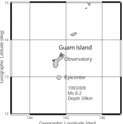
Fig. 1. Relative location of our ULF observing station and the
epi-center of the Guam earthquake, together with the earthquake char-acteristics.
in estimating the fractal dimension.
In this paper we intend to try to compare the results by the two different methods to the same ULF electromagnetic data including the 1993 August Guam EQ; (1) mono-fractal analysis (Ida et al., 2006) and (2) flicker noise spectroscopy (Hayakawa and Timashev, 2006). This kind of comparison of results by different methods as applied to the same data enable us to think of the reliability of the obtained results and to go to the definite conclusion on the process taking place in the lithosphere.
2 Experimental ULF data and Guam earthquake
The details of the ULF data for the Guam EQ have already been given in Hayakawa et al. (1999), but we have to re-peat only the important points as follows. The period of data analysis is from January, 1992 to the end of 1994 (to-tal three years). The Guam EQ with magnitude Ms=8.2, oc-curred on 8 August, 1993 at 08:34 UT suddenly and without any foreshocks. Its epicenter was located in the sea near the Guam island (geographic coordinates: 12.89◦N, 144.80◦E) as shown in Fig. 1, and its depth was 60 km. The Guam ob-servatory where the ULF data were recorded, is located at
∼65 km from the epicenter. We here comment on the sen-sitivity distance of seismogenic ULF emissions. Hayakawa and Hattori (2004) and Hayakawa et al. (2007) have summa-rized all of the previous ULF emissions, who have concluded that the distance of sensitivity of ULF emissions is
approx-imately 100 km even for an EQ with magnitude 7.0. Fig-ure 1 illustrates the relative location of our ULF observatory with respect to the epicenter. A regular magnetic observa-tion was maintained there using a three-axis ring-core-type fluxgate magnetometer (Hayakawa et al., 1996). Three com-ponents of magnetic variations were usually recorded on a digital cassette tape with a sampling rate of 1 s.
We analyze the data during the whole period of three years, and we analyze the data during daytime (LT=14:00–15:00), because Gotoh et al. (2004) have found that the most signifi-cant change in the mono-fractal dimension was observed for the Guam EQ during daytime. One hour data are treated, so that the number of data is 3600 points per day.
3 Fractal (mono) analysis
The method of mono-fractal analysis has been already de-scribed in details in Ida and Hayakawa (2006). Different kinds of methods of fractal behavior of time series data have been proposed, but we have used the Higuchi (1988) method, because Gotoh et al. (2003, 2004) have compared different methods extensively and have come to the conclusion that the Higuchi method is superior to others. The fractal dimen-sion defined and used by Higuchi is most reasonable and ac-ceptable in the sense of fractal definition. Here we explain briefly the Higuchi’s method. The estimation of fractal di-mension (D) of the time series data (in our case ULF data with sampling of 1 s) is based on the estimation of the length of the curveX(t ). The fractal time seriesX(t )of our con-cern is used to define the following new time series.
˜
Xm(k);X (m) , X (m+k) , X (m+2k) ,· · ·,
X
m+
N−m
k
·k
(m = 1, 2, · ··, k)
We estimate the curve length for eachX˜
m(k), and we call it.
Lm(k)(m=1, 2,· · ·,k).
Lm(k)=
h
N−m k
i
P
i=1
|X (m+ik)−X (m+(i−1)·k)|hN−1
N−m k
i ·k
k
where the term,(N−1)N−km·kis the normalizing fac-tor. Finally, the curve length is defied as the arithmetic aver-age as follow.
hL (k)i = k
P
m=1
Lm(k)
k
Then, we plothL (k)iversusk(k=1, 2,· · ·,kmax)(here we tentatively takekmax=10) and we estimate the slope by fitting, leading to the estimation of the mono-fractal dimension, D.
H component, so that the result for H component is plotted in Fig. 2. Figure 2 is the summary of the temporal evolution of mono-fractal dimension in the bottom panel. One result is obtained for one day, so that the thin line is the connection of those one-day results. While, the full line is the running average over±5 days. In order to indicate the statistical sig-nificance of the peaks in the fractal dimension, D, we have plotted the average value for the whole period (as a hori-zontal line) and the±σ (σ: standard deviation) lines. For the sake of comparison, the top panel illustrates the temporal evolution of geomagnetic activity expressed by Ap index.
4 Flicker noise spectroscopy method
This flicker noise spectroscopy which is a new phenomeno-logical method for the retrieval of information contained in chaotic time signals. The details of the method has already been described in Hayakawa and Timashev (2006) and Tima-shev (2001). According to this phenomenological approach, the main information hidden in a chaotic signal at an in-terval T is provided by sequences of distinguishing types of irregularities-spikes, jumps, and discontinuities of deriva-tives of different orders at all space-time hierarchical levels of systems. It is possible to introduce different types of in-formation. The ability to distinguish the irregularities means that the parameters or patterns characterizing the totality of properties of the irregularity sequences, are extracted from the following power spectraS(f )(f, frequency).
S (f )=
T/2 Z
−T/2
hX (t ) X (t+t1)·exp(2π if t1) dt1i
,
h(· · ·)i = 1
T
T/2 Z
−T/2
(· · ·) dt ,
and the difference moments8(2)(τ) of the 2nd order,
8(2)(τ )= hX (t )−X (t+τ )i2=
*
t+τ
Z
t
dX (x) dx
2
+
,
whereτ is time delay. In this case,8(2)(τ) is formed exclu-sively by jumps of the dynamic variable different space-time hierarchical levels of the system under consideration, andS
(f )is formed by spikes and jumps. In other words, the power spectra and difference moments of the 2nd order carry differ-ent information, which complemdiffer-ent each other. The charac-teristic are the “passport parameters”, which are the correla-tion times, parameters characterizing the loss of “memory” for these correlation times, characterizing the sequences of “spikes”, “jumps” and discontinuities of derivatives of dif-ferent orders.
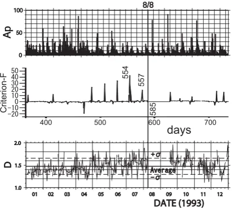
Fig. 2. Comparison of the results by the two analysis methods; (1)
2nd panel is the result by the flicker noise spectroscopy and the bottom panel, that by the mono-fractal analysis (fractal dimension). The top panel indicates the Ap index.
In the most real cases, S (f ) and 8(2) (τ) depen-dences manifest their complexity and non-stationary behav-ior. Then, the introduction of “passport parameters” to de-scribe the temporal evolution is useless. At the same time, the behavior of the realS (f )and8(2) (τ) is very specific and individual to each study case. These dependences have a definite physical sense and characterize the sequences of spikes, jumps and discontinuities of derivatives of different orders. That is why these dependences can be considered as “characteristic passport patterns” of the evolution under study.
While studying non-stationary processes, dynamics of the
S(f )and8(2)(τ) variations is being analyzed at sequential shift of the averaging interval [k1T,tk] with the extension
T, wherek= 0, 1, 2, 3· · ·andtk=T+k1T, for the value1T
along the whole time intervalTtot(T+1T < Ttot)of the avail-able experimental data. The time intervalsT and1T should be selected as based on the physical sense of the considered problem - revealing the typical time of a process which deter-mines the most important internal structural reconstruction of the studied evolution.
It is obviously natural to associate a phenomenon of “pre-cursor” occurrence with the sharper variations of the rela-tionsS(f )and8(2)(τ) at the approach of the upper bound-ary of the time interval of averagingtk to a momenttcof a
catastrophic event when reconstruction takes place at all the possible spatial scales in the system. It is also natural to ex-pect (in this case we may speak about a “precursor”) that the time of the “precursor’s” manifestationtk should stand from
tk≥1T, at realization of the inequality1Tcn<< Tt ot. When
revealing a “precursor”, it is important to distinguish cases when sharp variations inS(f )and8(2)(τ) at averaging in-tervalT shift are caused by significant signal variations on the “front” or “back” boundary of the interval T by approach-ing the “front” boundarytk to a momenttc of the expected
event. A given problem is being solved by the analysis of the time behavior of the corresponding criteria at theT vari-ations: it is obvious that whenT increases in a value1T1the non-stationary effects associated with the signal behavior at the “back” boundary should be displayed with the same time delay1T1, when the factor display caused by sharp signal variations in the area of the front boundary does not depend so strongly on the average interval value. Next we consider the “precursors” that are defined by the difference moments
8(2)(τ). These functions can be reliably calculated only for a delayτ in the range [0,αT] withα≤0.5. Let us introduce the dimensionless quantities:
C (tk+1)=2·
Qk+1−Qk
Qk+1+Qk
1T
T ;
Qk = αT
Z
0 h
8(2)(τ )i
kdτ.
Here tk+1=k1T(k=0, 1, 2, · · ·)and subscripts of square brackets show that8(2) (τ) dependence was calculated for time interval [k1T, k1T+T]. The quantities introduced characterize a measure or factor of non-stationarity of the signals, as the averaging intervalT moves along time axis by a step1T. In particular, when the “forward” boundary of the averaging intervaltkapproaches the catastrophic event at
timetc, evidentlyC (tk+1)=0 for the stationary processes at
T→∞.
We use the “high-frequency” components of the signals (CF), because the criterion factors CF (tk) demonstrated
clearer results as compared to the low-frequency CG (tk).
The problem is to reveal the non-stationary factors and to understand whether these factors could be considered as pre-cursors of the earthquake.
The initial second data were used to get the initial minute data; every 60th second data were taken. Then we formed the hourly data (every 60th reading of the minute time se-ries) as well as the daily time series (formed by every 24th reading of the hour time series). At first, we began to analyze the daily data. It is well known that large EQs are prepared during several years. That is why we began our analysis by considering large T-intervals for finding a precursor for the case of M=8.2. In this case we processed the daily time se-ries and calculated theCF(tk)factors by choosing T=550,
500, 400, 300, 200 and 100 days as well as1T = 1 day for all cases. The results are calculated forT=550 (500, 400, 300, 200, and 100) days, and1=1 day, but we present only one example among them in Fig. 2 with T=300 days and
1T=1 day. Many large peaks are found to be present in the calculated dependences as in Fig. 2. The appearance of every peak at different meanings of the current time means that the state of the geophysical medium is changed at these times. If anyone considers an ordinary time series (for the Z or other components) the appearance of any peak means that the measured value drops after rising. That is all. But in the case of the flicker noise spectroscopy non-stationary cri-teria the appearance of every peak means that the state of the medium is different before and after the peak. It means that the seismo-active medium could be reconstructed (changes its state) several times before the EQ. It is interesting to study the dynamics of the realized peaks during the whole time (3 years in our case). We can notice five significant peaks in
CF in Fig. 2 before the large EQ located on the day of 585
(Guam EQ), which will be our greatest concern below. It is possible to think that the 5 peaks many reflect the 5 stages of the complex processes of the medium rearrangement be-fore the coming catastrophic EQ. These precursors appeared at 101, 78, 54, 31 and 8 days before the EQ.
5 Comparison of both results
As is already shown by Smirnova and Hayakawa (2007), the main part of the ULF signals is of magnetospheric origin, so that we have to pay attention to the temporal evolution of Ap index in the top panel of Fig. 2. Smirnova and Hayakawa (2007) have shown that the SOC process is also taking place before a major geomagnetic storm, just in the case of EQs. The geomagnetic activity during the period when we notice several peaks inCF and D plots (during 4 months before the
EQ), is found to be relatively quiet, so that we do not expect any SOC process in the Earth’s magnetosphere.
The result by the flicker noise spectroscopy is summarized in the second panel of Fig. 2 in the form of temporal evolu-tion ofCF (criterion-F) factor just around the Guam
earth-quake (8 August 1993; Day=585d). This analysis is done withT=300 days and 1T=1 day. It is possible for us to identify significant peaks in the CF factor evolution; that is,
these peaks appeared 101, 78, 54, 31 and 8 days before the EQ. This is indicative of the 5 stages of the complex process of the medium rearrangement before the coming catastrophic EQ. The result by the flicker noise spectroscopy provides us with spiky results, while the mono-fractal analysis (in the bottom of Fig. 2) gives us the continuous variation. How-ever, as you can see from the bottom panel of Fig. 2, we note that the fractal dimension (D) exhibits a significant change from the end of April, 1993 in such a way that the fractal dimension is notably increased from the end of April. This transition time is coincident with the time of the first spike in theCF factor (101 days before the EQ), and the period for
comparison by two methods is that the running curve of the mono-fractal dimension exhibits several maxima, whose po-sitions are generally coincident with the peaks found by the flicker noise spectroscopy. Another point we have to pay at-tention is the period between the 4th peak (31 days before the EQ) and the EQ. While, the fractal dimension is seen to remain at a rather high value with large fluctuations. After the EQ, the fractal dimension is seen to show a tendency of decrease toward the pre-EQ level in December, 1993 or so. The general conclusion as based on the extensive comparison of results by the two methods, can be drawn as follows;
1. Only one year data (January to December, 1993) are presented in Fig. 2, though we have analysed±1.5 years around the EQ. It is clear from the results by both meth-ods that some significant effects have definitely taken place just around the EQ.
2. Some precursory effects seem to start about 3 months before the EQ, and re-arrangement of the lithospheric medium seems to be taking place 3 months before the EQ and a few months even after the EQ.
3. Both analysis methods have yielded very consistent re-sults on the precursory behavior taking place in the lithosphere in the period from 3 months before the EQ up to the EQ. The flicker noise spectroscopy indicates that there are 5 peaks before the EQ (101, 78, 54, 31 and 8 days before the EQ), and during this period of those peaks the mono-fractal dimension, D is found to be significantly enhanced.
4. Several peaks in the flicker noise spectroscopy result might indicate the step-like changes in the lithosphere just before the EQ due to the self-organization critical-ity process.
Acknowledgements. The original ULF data were made available
to us by K. Yumoto of Kyusyu University, whom we would like to thank. One of the authors (M. Hayakawa) would like to express his sincere thanks to NiCT (R&D promotion scheme funding international joint research) for its support. This work is also supported by Russian Fund of Fundamental Research (grant 05-02-17079), to which S. Timashev is grateful.
Edited by: P. F. Biagi
Reviewed by: two anonymous referees
References
Bak, P., Tang, C., and Wiesenfeld, K.: Self-organized criticality: An explanation of 1/fnoise, Phys. Rev. Lett., 59, 381–384, 1987. Bak, P.: How Nature works (The Science of Self-organized
Criti-cality), Oxford University Press, 201 pp, 1997.
Burlaga, L. F. and Klein, L. W.: Fractal structure of the interplane-tary magnetic field, J. Geophys. Res., 91, 347–350, 1986.
Fraser-Smith, A. C., Bernardi, A., McGill, P. R., Ladd, M. E., Hel-liwell, R. A., and Villard Jr., O. G.: Low-frequency magnetic field measurements near the epicenter of the Ms 7.1 Loma Prieta earthquake, Geophys. Res. Lett., 17, 1465–1468, 1990. Gotoh, K., Hayakawa, M., and Smirnova, N.: Fractal analysis of
the ULF geomagnetic data obtained at Izu peninsula, Japan in relation to the near by earthquake swarm of June-August 2000, Nat. Hazard Earth Syst.Sci., 3, 229–236, 2003.
Gotoh, K., Smirnova, N., and Hayakawa, M.: Fractal analysis of seismogenic ULF emissions, Special Issue on “Seismo Electro-magnetics and Related Phenomena”, edited by: Hayakawa, M., Molchanov, O. A., Biagi, P., and Vallianatos, F., Phys. Chem. Earth, Parts A/B/C, 29(4–9), 419–424, 2004.
Hayakawa, M. (Ed.): Atmospheric and Ionospheric Electromag-netic Phenomena Associated with Earthquakes, Terra Sci. Pub. Comp., Tokyo, pp. 996, 1999.
Hayakawa, M., Molchanov, O. A., and NASDA/UEC Team: Sum-mary report of NASDA’s earthquake remote sensing frontier project, in: Special Issue on Seismo Electromagnetic and Re-lated Phenomena, edited by: Hayakawa, M., Molchanov, O. A., Biagi, P., and Vallianatos, Phys. Chem. Earth, 29(4–9), 617–626, 2004.
Hayakawa, M., Itoh, T. and Smirnova, N.: Fractal analysis of ULF geomagnetic data associated with the Guam earthquake on Au-gust 8, 1993, Geophys. Res. Lett., 26, 2797–2800, 1999. Hayakawa, M., Itoh, T., Hattori, K., and Yumoto, K.: ULF
elec-tromagnetic precursors for an earthquake at Biak, Indonesia on February 17, 1996, Geophys. Res. Lett., 27, 1531–1534, 2000. Hayakawa, M.: NASDA’s Earthquake Remote Sensing Frontier
Research, Seismo- electromagnetic Phenomena in the Litho-sphere, Atmosphere and IonoLitho-sphere, Final Report 228 p, Univ. of Electro-Communications, March, 2001.
Hayakawa, M. and Fujinawa, Y.: Electromagnetic Phenomena Re-lated to Earthquake Prediction, Terra Sci. Pub. Comp., Tokyo, Japan, pp. 477, 1994.
Hayakawa, K., Kawate, R., Mochanov, O. A., and Yumoto, K.: Re-sults of ultra-low-frequency magnetic field measurements during the Guam earthquake of 8 August 1993, Geophys. Res. Lett., 23, 241–244, 1996.
Hayakawa, M. and Molchanov, O. A. (Eds.): Seismo Electromag-netics : Lithosphere – Atmosphere – Ionosphere Coupling, TER-RAPUB, Tokyo, pp. 477, 2002.
Hayakawa, M. and Hattori, K.: Ultra-low-frequency electromag-netic emissions associated with earthquakes, Inst. Electr. Engrs. Japan, Trans. Fundamentals and Materials, 124(12), 1101–1108, 2004.
Hayakawa, M. and Timashev, S. F.: An attempt to find precursors in the ULF geomagnetic data by means of flicker noise spec-troscopy, Nonlin. Processes Geophys., 13, 255–263, 2006, http://www.nonlin-processes-geophys.net/13/255/2006/. Hayakawa, M., Hattori, K., and Ohta, K.: Monitoring of ULF
(ultra-low-requency) geomagnetic variations associated with earth-quakes, Sensors, 7, 1108–1122, 2007.
Higuchi, T.: Approach to an irregular time on the basis of fractal theory, Physica D, 31, 277–283, 1988.
the 1993 Guam earthquake to study prefecture criticality, Nonlin. Process Geophys., 13, 409–412, 2006.
Kapiris, P. G., Balasis, G. T., Kopanas, J. A., Antonopoulos, G. N., Pertezakis, A. S., and Eftaxias, K. A.: Scaling similarities of multiple fracturing of solid materials, Nonlin. Process Geophys., 11, 137–151, 2004.
Kopytenko, Y. A., Matishvili, T. G., Voronov, P. M., Kopytenko, E. A., and Molchanov, O. A.: Detection of ultra-low-frequency emissions connected with the Spitak earthquake and its after-shock activity, based on geomagnetic pulsations data at Dusheti and Vatdzia observations., Phys. Earth Planet. Inter., 77, 85–95, 1993.
Molchanov, O. A., Kopytenko, Y. A., Voronov, P. M., Kopytenko, E. A., Matiashvill, T. G., Fraser-Smith, A. C., and Bernardi, A.: Results of ULF magnetic field measurements near the epicen-ters of the Spitak (ms=6.9) and Loma Prieta (Ms=7.1) earth-quakes: Comparative analysis, Geophys. Res. Lett., 19, 1495– 1498, 1992.
Molchanov, O. A. and Hayakawa, M.: Generation of ULF electro-magnetic emissions by microfracturing, Geophys. Res. Lett., 22, 3091–3094, 1995.
Vallianatos, F. and Tzanis, A.: A model for the generation of precursory electric and magnetic fields associated with the de-formation rate of the earthquake focus, in “Atmospheric and Ionospheric Electromagnetic Phenomena Associated with Earth-quakes”, edited by: Hayakawa, M., TERRAPUB, Tokyo, 287– 306, 1999.
Smirnova, N., Hayakawa, M., Gotoh, K., and Volobuev, D.: Scaling characteristics of ULF geomagnetic field at the Guam seismoac-tive area and their dynamics in relation to the earthquake, Nat. Hazards Earth Syst. Sci., 1, 119–126, 2001
Smirnova, N. A. and Hayakawa, M.: Fractal characteristics of the ground-observed ULF emissions in relation to geomagnetic and seismic activities, J. Atmos. Solar-Terr. Phys., in press, 2007. Timashev, S. F.: Flicker-noise spectroscopy as a tool for analysis of
fluctuations in physical system, Noise in Physical Systems and 1/f Fluctuations, World Scientific, edited by: Bosman, G., World Scientific, 775–778, 2001.