Themed Section: Science and Technology
A Meta-Stacked Software Bug Prognosticator Classifier
Ajay Kumar Shrivastava*1, Dr. Ekbal Rashid2
*1M.Tech Research Scholar, Jharkhand Rai University, Ranchi, Jharkhand, India
2Department of CSE, Aurora’s Technological and Research Institute, Uppal, Hyderabad, Telangana, India
ABSTRACT
Predicting defects defines the proactive process of classifying the defects that can be found in entire software’s content, within and cross-project codes for producing high quality product with optimized cost. Error prediction in open source software is more crucial due to its inherent complexity and the large repository of contributors. In this paper we present the meta-stacked regression model (MSRM) which improvises the Rayleigh Probabilistic distribution for feature selection estimates. Firstly, a heuristic bug mining approach is adopted to mine the parameters reported by developers and contributors of various Open source projects (Bugzilla, Eclipse, Mozilla) activity logs. In the second part, Stacked Regression is compared to Neural Networks and Linear Support Vector Machine models in terms of the bug prediction performance with Feature importance and Correlation amongst parameters. The results show that the ensemble based Stacked regression has better precision and F-measure compared to simple machine learning models. The MSRM model accurately predicts and classifies bugs with accuracy of 96.8% and reduces the impact of false positives by recall of 71.2%. Keywords: Stacked Regression, Bug Prediction, Cost Estimation, Rayleigh defect density, Software Project Bugs
I.
INTRODUCTION
The occurrence of bugs is a deterrent in any software project cost estimation and directly affects the quality and success of any software management. It can affect macroscopic elements like resource allocation, project planning and bidding, as well as micro-level phase wise design and execution hence bug estimation at an early stage of software testing has led to extensive research efforts. Bugs can reduce the reliability of a software system affecting its estimation and model accuracy. Boehm’s constructive cost model COCOMO and COCOMO II [3], Albrecht’s function point method [2] and Putnam’s software life cycle management (SLIM) [15] are the initial algorithmic estimation methods which were used for software estimation by Constructive Cost Model is by far the most commonly used because of its simplicity for estimating the effort in person-month for a project at different stages.
The remainder of this paper is organized as follows: Sect. II discusses about the related literature review and its shortcomings. Section III discusses about the methods involved in implementing the various meta-classifiers.
Section IV discusses the proposed MSRM process flow on various classifiers. Section V discusses the results and paves way for further research.
II.
RELATED WORK
Barry Boehm et.al [3](2000) addressed on an overview of a variety of software estimation models indicating that neural-net and dynamics-based techniques are less mature than the other classes of techniques and are challenged by the rapid changes in software technology. The key to arriving at sound estimates is to have a grasp of the factors which are driving the costs of the project at hand to support the project planning and control functions performed by the management.
S.Wang et.al [2](2016) proposed to bridge the gap between programs’ semantics and defect prediction features by representation-learning algorithm. Deep Belief Network (DBN) was adopted to learn semantic features from token vectors extracted from programs’ Abstract Syntax Trees (ASTs) and evaluated on ten open source projects. Results showed improvement in WPDP 14.7% in precision, 11.5% in recall, and 14.2% in F1. For CPDP, the semantic features based approach outperforms the state-of-the-art technique TCA+ with traditional features by 8.9% in F1 score.
The first contribution of our work is to find the set of priority attributes that affect the cost of bug estimation the most. Second is to evaluate the stacked classifiers (Regression, Neural Network, Linear SVM) with density distribution in terms of prediction accuracy and F1 score.
III.
METHODOLOGY
Feature selection aims to find a Q-dimensional subset of features, Set Q, (QF) that optimizes classifier performance and optionally minimizes the feature set size. The primary reasons to use feature selection are that it enables the machine learning algorithm to train faster, improves the accuracy of a model with the right subset and it substantially reduces over fitting. With a carefully chosen set A ⊂ R, we can classify a new data point x ∈ R d by checking whether f(x) ∈ A.
3.1 Logistic Regression Model
The regression model considered for classification of bug occurrence can be written in the form
For n independent pairs (xi, yi), i=1,2,.. n where
x’i =(x0i,x1i..., xni). For the outcome Yi, the logistic regression model assumes that
P(Yi=1 for xi) = µ(xi) ...(i) where µ(xi)=eg(xi)/ (1 + eg(xi)) with g(xi)=x’iß...(ii) The maximum likelihood is obtained for parameter estimates and the fitted values are specified as
µ’(xi) = µ(xi, ß) i.e. logit[µ (x)]= x’ ß...(iii)
3.2 Linear Support Vector Model
Linear Classifiers define the margin as the width that the boundary could be increased by before hitting a datapoint. Support Vectors are those data points that the margin pushes up against linear classifier with the maximum margin. This is called LSVM.
Figure 1. Linear Support Vectors as function of weight and bias
The linear objective is expressed as
The corresponding goal of weights and bias is given as w =Σαiyixi ; b= yk- wTxk………...(v) for any xk such that αk 0 .Here, each non-zero αi indicates that corresponding xi is a support vector and classifying function will have the form
ℱ (x) = ΣαiyixiTx + b...(vi)
3.3 Radial Basis Function Neural network Model The objective of Neural system is to find a progression of weights that will give important values in the yield when determined particular cases of its information. Each node in hidden layer gain input from the input layer, which are multiplexed with proper weights and reduced.
Figure 2. The mathematical analogy of ANN with synaptic structure of Neural Systems with output f(x)
3.4 Rayleigh’s Density Distribution
The Rayleigh distribution[6] is a special case of the Weibull distribution, which provides a population model useful in several areas of statistics, including life testing and reliability study. Rayleigh distribution RD (Ø) is employed in parameter estimation using different types of censoring and non-censoring data and written as :-
Probability Distribution Function (PDF) = 2 * Øx*e-Øx2 where x>0 and Ø>0...(vii) Also Cumulative Distribution Function (CDF) = 1-e-Øx2 ...(viii)
IV.
PROPOSED FRAMEWORK
In this paper the following steps were taken in the process of model building of MSRM :-
1 ) Data Extraction
The bug reports of different products of Eclipse, Mozilla and Bugzilla [5]open source software were retrieved from the CVS repository and saved in .csv format from source : http://bugzilla.mozilla.org 2) Data Pre-Processing & Preparation
Remove missing and Noisy data by setting all non zero value to 1 for depends on and duplicate count attributes. Divide the Dataset into Training data for Model creation and testing data for validation (60:40).
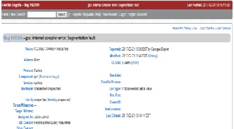
Figure 3. A Sample Bug report for Open Office Project with BugID 1425569
3) Modeling
Build three models based on LSVM, RBNN classifiers and Regression model.
Calculate the summary weight of bug attributes by using information gain criteria. Train the Model by using most relevant twelve attributes to predict and the bug severity.
Apply Rayleigh probability density to predict defect density for different phases of project life cycle. 4) Testing and Validation
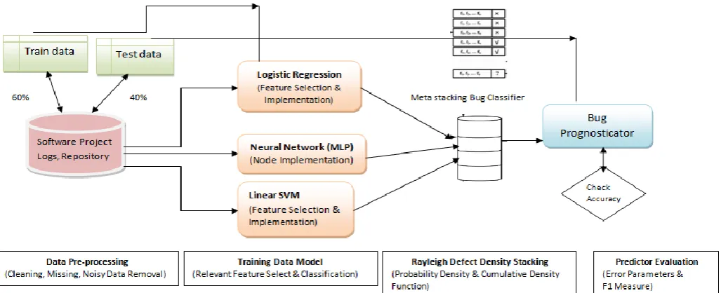
Figure 4. Overview of our proposed MSRM for defect prediction
Several experiments were conducted by recording the bug repository to study the performance of the proposed stacked model in comparison with existing classifiers. The experiments were run on a 2.5GHz i5-3210M machine with 4GB RAM.
To measure defect prediction results, we use four Evaluation metrics: Correlation, Precision, Recall, and F1score[3].
Pearson’s Correlation: It is used as a measure for quantifying linear dependence between two continuous variables X and Y. Its value varies from -1 to +1. Pearson’s correlation is given as:
Y X Y
X
Y X
, cov ,...(ix)
F-measure: Weighted (by class size) average F-measure was obtained from the classification using feature subset with the same three classifiers as above. It describes the Harmonic mean of Precision and Recall.
The general formula for positive real β is given by;
recall ecision
recall ecision
F
) Pr
( Pr
1 2 2
...(x)
FP TP
TP precision
...(xi)
FN TP
TP recall
...(xii)
Here Precision is the ratio of all relevant correctly classified bugs to all retrieved bugs.
Recall is measured as the fraction of relevant items retrieved out of all relevant items including False data not correctly classified.
V.
RESULTS AND DISCUSSION
Figure 5. Bug Attributes Selected by Feature Importance Graph
Figure 6. Correlation Graph for Most relevant Feature Selection
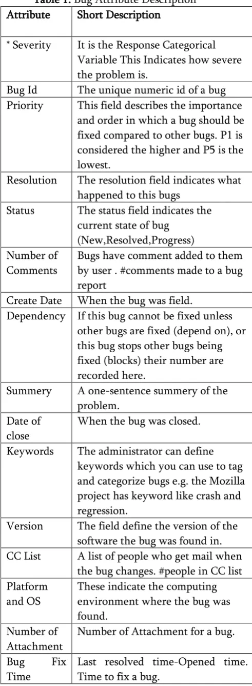
Table 1. Bug Attribute Description Attribute Short Description
* Severity It is the Response Categorical Variable This Indicates how severe the problem is.
Bug Id The unique numeric id of a bug Priority This field describes the importance
and order in which a bug should be fixed compared to other bugs. P1 is considered the higher and P5 is the lowest.
Resolution The resolution field indicates what happened to this bugs
Status The status field indicates the current state of bug
(New,Resolved,Progress) Number of
Comments
Bugs have comment added to them by user . #comments made to a bug report
Create Date When the bug was field.
Dependency If this bug cannot be fixed unless other bugs are fixed (depend on), or this bug stops other bugs being fixed (blocks) their number are recorded here.
Summery A one-sentence summery of the problem.
Date of close
When the bug was closed.
Keywords The administrator can define keywords which you can use to tag and categorize bugs e.g. the Mozilla project has keyword like crash and regression.
Version The field define the version of the software the bug was found in. CC List A list of people who get mail when
the bug changes. #people in CC list Platform
and OS
These indicate the computing environment where the bug was found.
Number of Attachment
Number of Attachment for a bug.
Bug Fix Time
Next, Stacking was performed by applying Rayleigh defect density on generating the mean probabilities of the classifiers hence further performance tuning led to the improved accuracy of the testing dataset as compared to the individual classifiers. Figures 7-9 depict the results of proposed MSRM model applied on 204545 bugs to depict the F1 Score.
Figure 7. Bug Reports on Severity Parameter for Eclipse
Figure 8. Severity Classification for Mozilla Product
Figure 8. No. Of bugs Correctly classified for Bugzilla with Severity Prediction.
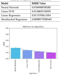
The final evaluation metric is to compute the error in prediction by the stacked regression Model(MSRM) as compared to the NN, LSVM and Linear regression Model.
Root mean squared error (RMSE): RMSE is a quadratic scoring rule that also measures the average magnitude of the error. It’s the square root of the average of squared differences between prediction and actual observation.
...(xiii) The RMSE values as calculated on the bug dataset classification and prediction was
Table 2. Comparative Error Estimates
Model RMSE Value
Neural Network 0.0184908700285 Linear SVM 0.0136835156595 Linear Regression 0.0115793611054 MetaStacked Regression 0.00989779285401
Figure 8. Comparative Predictive error of MSRM Model.
VI.
CONCLUSION
Future enhancements include adopting the MSRM model for web-based and component-based software data sets.
VII.
REFERENCES
[1]. X. Huo, M. Li, and Z.-H. Zhou, "Learning unified features from natural and programming languages for locating buggy source code," in Proceedings of IJCAI'2016
[2]. S. Wang, T. Liu, and L. Tan, "Automatically learning semantic features for defect prediction," in ICSE'16: Proc. of the International Conference on Software Engineering, 2016 [3]. V. Raychev, M. Vechev, and E. Yahav, "Code
completion with statistical language models," in ACM SIGPLAN Notices, vol. 49, no. 6. ACM, 2014, pp. 419-428.
[4]. Jian Li, Pinjia He, Jieming Zhu, and Michael R. Lyu.2017. "Software Defect Prediction via Convolutional Neural Network" at IEEE International Conference on Software Quality, Reliability and Security, 2017
[5]. Z. He, F. Peters, T. Menzies, and Y. Yang, "Learning from open-source projects: An empirical study on defect prediction," in ESEM'13: Proc. of the International Symposium on Empirical Software Engineering and Measurement, 2013.
[6]. N. A. Abou-Elheggag, Estimation for Rayleigh distribution using progressive first-failure censored data, Journal of Statistics Applications and Probability 2(2) (2013) 171-182.
[7]. J. Wang, B. Shen, and Y. Chen, "Compressed c4. 5 models for software defect prediction," in QSIC'12: Proc. of the International Conference on Quality Software, 2012.
[8]. T. Gyimothy, R. Ferenc, I. Siket, "Empirical Validation of Object-Oriented Metrics on Open Source Software for Fault Prediction", IEEE Transactions on Software Engineering, vol. 31, no.10, pp. 897-910, 2005.
[9]. S.W. Haider, J.W. Cangussu, K.M.L. Cooper, R. Dantu, "Estimation of Defects Based on Defect Decay Model: ED3M", IEEE Transactions on Software Engineering, vol. 34, no. 3, pp. 336-356, 2008.
[10]. R. M. El-Sagheer, Inferences using type-II progressively censored data with binomial removals, Arabian Journal of Mathematics 4 (1) (2015) 127-139.