Understanding Surface Hopping Algorithms And Their Applications In Condensed Phase Systems

University of Pennsylvania

ScholarlyCommons

Publicly Accessible Penn Dissertations

2017

Understanding Surface Hopping Algorithms And

Their Applications In Condensed Phase Systems

Wenjun Ouyang

University of Pennsylvania, [email protected]

Follow this and additional works at:https://repository.upenn.edu/edissertations Part of thePhysical Chemistry Commons

Recommended Citation

Ouyang, Wenjun, "Understanding Surface Hopping Algorithms And Their Applications In Condensed Phase Systems" (2017). Publicly Accessible Penn Dissertations. 2508.

Understanding Surface Hopping Algorithms And Their Applications In

Condensed Phase Systems

Abstract

While electron transfer plays an important role in a variety of fields, our understanding of electron transfer relies heavily on quantum mechanics. Given the high computational cost of quantum mechanics calculations and the limits of a computer's capability nowadays, the straightforward use of the Schrodinger equation is extremely limited by the dimensionality of the system, which has spurred the advent of many approximate methods. As a mixed quantum-classical approach, fewest-switches surface hopping (FSSH) can treat many nuclei as classical particles while retaining the quantum nature of electrons. However appealing, though, FSSH has some notable drawbacks: FSSH suffers from over-coherence (in addition to its inability to capture presumably rare nuclear quantum effects). Here, in this thesis, we revisit the issue of decoherence from the perspective of entropy, unraveling the nature of the erroneous coherence associated with FSSH trajectories and further justifying the improvements made by the recently proposed augmented-FSSH. Going beyond traditional Tully-style surface hopping technique, we also study new flavors of surface hopping that treat a manifold of electronic states to capture dynamics near metal surfaces. Moreover, we highlight how surface hopping can be used to study electrochemistry and we thoroughly benchmark the surface hopping algorithms against mean-field approaches. This thesis captures 4 years of research which has successfully analyzed the guts of the surface hopping approach for nonadiabatic dynamics both in solution and at a metal surface.

Degree Type

Dissertation

Degree Name

Doctor of Philosophy (PhD)

Graduate Group

Chemistry

First Advisor

Joseph E. Subotnik

Keywords

Anderson-Holstein model, decoherence, electrochemistry, electron transfer, mixed quantum-classical approach, surface-hopping

Subject Categories

UNDERSTANDING SURFACE HOPPING ALGORITHMS AND THEIR

APPLICATIONS IN CONDENSED PHASE SYSTEMS

Wenjun Ouyang

A DISSERTATION

in

Chemistry

Presented to the Faculties of the University of Pennsylvania

in

Partial Fullfillment of the Requirements for the

Degree of Doctor of Philosophy

2017

Supervisor of Dissertation

Dr. Joseph E. Subotnik

Professor of Chemistry

Graduate Group Chairperson

Dr. Gary A. Molander

Hirschmann-Makineni Professor of Chemistry

Dissertation Committee

Dr. Andrew M. Rappe, Blanchard Professor of Chemistry

DEDICATION

To my parents for their love and support that raises me up.

To my wife without whom I could not survive the difficulties along the way and

ACKNOWLEDGMENT

I would like to thank my advisor Dr. Joseph Subotnik whom it is my greatest

for-tune and honor to work with. His support and help in both my research and life

has been invaluable in these unforgettable five years’ experience as an international

student. He is knowledgeable and willing to teach and help me with the best of his

expertise when I stumbled in my research. He is accommodating and creates a great

environment for everyone in the group. His enthusiasm in science has inspired me to

learn more and deeper. His critical thinking has motivated me to think differently

and comprehensively. Going through five years for the Ph.D. is definitely not easy,

but Dr. Subotnik has made it tractable and enjoyable and more meaningful.

I would also like to thank my dissertation committee: Dr. Andrew Rappe, Dr.

Marsha Lester and Dr. Michael Topp. It is my great pleasure to be able to have

them in my committee and they have provided me with invaluable advice along the

way to today. Without them, I could not have been as successful today.

My sincere gratitude goes to the Subotnik’s group as well: Dr. Brian Landry,

Dr. Ethan Alguire, Dr. Xinle Liu, Dr. Andrew Petit, Dr. Amber Jain, Dr. Greg

Medders, Qi Ou, Wenjie Dou, Nicole Bellonzi, Zuxin Jin, and Gaohan Miao. It is

my great fortune to be able to work with these very smart and nice people. Their

ABSTRACT

UNDERSTANDING SURFACE HOPPING ALGORITHMS AND THEIR

APPLICATIONS IN CONDENSED PHASE SYSTEMS

Wenjun Ouyang

Dr. Joseph E. Subotnik

While electron transfer plays an important role in a variety of fields, our

under-standing of electron transfer relies heavily on quantum mechanics. Given the high

computational cost of quantum mechanics calculations and the limits of a computer’s

capability nowadays, the straightforward use of the Schr¨odinger equation is extremely

limited by the dimensionality of the system, which has spurred the advent of many

approximate methods. As a mixed quantum-classical approach, fewest-switches

sur-face hopping (FSSH) can treat many nuclei as classical particles while retaining the

quantum nature of electrons. However appealing, though, FSSH has some notable

drawbacks: FSSH suffers from over-coherence (in addition to its inability to capture

presumably rare nuclear quantum effects). Here, in this thesis, we revisit the issue of

decoherence from the perspective of entropy, unraveling the nature of the erroneous

coherence associated with FSSH trajectories and further justifying the improvements

made by the recently proposed augmented-FSSH. Going beyond traditional

Tully-style surface hopping technique, we also study new flavors of surface hopping that

treat a manifold of electronic states to capture dynamics near metal surfaces.

More-over, we highlight how surface hopping can be used to study electrochemistry and we

thoroughly benchmark the surface hopping algorithms against mean-field approaches.

This thesis captures 4 years of research which has successfully analyzed the guts of

LIST OF CONTENTS

DEDICATION ii

ACKNOWLEDGMENT iii

ABSTRACT iv

LIST OF ILLUSTRATIONS ix

CHAPTER 1 Introduction 1

CHAPTER 2 Estimating the Entropy and Quantifying the Impurity

of a Swarm of Surface-Hopping Trajectories: A New Perspective on

Decoherence 12

2.1 Introduction . . . 12

2.2 Background: The Entropy of a Wigner Wavepacket on One Electronic Surface . . . 16

2.3 The Impurity of a Partial Wigner Wavepacket on Multiple Electronic Surfaces . . . 17

2.3.1 Exact Dynamics from the Schr¨odinger Equation . . . 18

2.3.2 The Quantum-Classical Liouville Equation (QCLE) . . . 20

2.3.3 FSSH Algorithm and the Calculation of Impurity . . . 22

2.4 Results . . . 24

2.4.1 Tully Problem #1: Avoided Crossing . . . 26

2.4.2 Tully Problem #3: Extended Couplings . . . 31

2.4.3 Impurity . . . 40

2.5.1 Exact Quantum Dynamics Predicts Nonlocal Coherences and

Phase Oscillations . . . 44

2.5.2 FSSH Predicts Local Coherences: An Analytical Measure of FSSH Impurity . . . 46

2.5.3 The Efficiency of FSSH Comes at the Expense of Ignoring Re-coherences and Not Conserving Impurity . . . 49

2.6 Conclusions . . . 51

2.7 Acknowledgments . . . 52

CHAPTER 3 Surface Hopping with a Manifold of Electronic States I: Incorporating Surface-Leaking to Capture Lifetimes 53 3.1 Introduction . . . 53

3.2 Surface-Leaking FSSH . . . 55

3.2.1 Tully’s Fewest-Switches Surface Hopping . . . 55

3.2.2 Surface-Leaking Algorithm . . . 57

3.2.3 SL-FSSH . . . 59

3.3 Results . . . 62

3.3.1 Model #1: One System State Couples to a Set of Nonparallel Bath States . . . 64

3.3.2 Model #2 and #3: Two System States With One Couples to a Set of Bath States . . . 73

3.4 Discussion . . . 75

3.4.1 Decoherence: Averaging over an Initial Wigner Wavepacket . . 75

3.4.2 The Mass Dependence of the Bath Dynamics . . . 79

3.4.3 Wide Band Approximation . . . 83

CHAPTER 4 A Surface Hopping View of Electrochemistry:

Non-Equilibrium Electronic Transport through an Ionic Solution with a

Classical Master Equation 90

4.1 Introduction . . . 90

4.2 Theory . . . 94

4.2.1 The Model Hamiltonian . . . 94

4.2.2 Boundary Conditions and Electron Transfer . . . 98

4.2.3 Algorithm . . . 100

4.2.4 Linear Response Theory . . . 102

4.3 Atomistic Details . . . 104

4.4 Results . . . 105

4.4.1 I-V Curve . . . 106

4.4.2 Position of Charged Solute (B−) Atoms . . . 110

4.4.3 Position of Electron Transfer . . . 113

4.5 Discussion . . . 118

4.5.1 Nonlinearity and Electron Transfer . . . 118

4.5.2 Interfacial Reaction . . . 122

4.6 Conclusions and Future Directions . . . 124

4.7 Acknowledgments . . . 126

CHAPTER 5 The Dynamics of Barrier Crossings for the General-ized Anderson-Holstein Model: Beyond Electronic Friction and Con-ventional Surface Hopping 127 5.1 Introduction . . . 127

5.2 Theory . . . 130

5.3 Results and Discussion . . . 135

5.3.1 Parabolic Diabats . . . 135

5.3.2 Electronic Friction for Small Γ . . . 137

5.3.3 Quartic versus Quadratic Diabatic Potentials . . . 139

5.4 Conclusions . . . 141

5.5 Acknowledgments . . . 142

CHAPTER 6 Conclusions 143

APPENDIX A 1D Exact Quantum Scattering Calculation 146

LIST OF ILLUSTRATIONS

1.1 Schematic figure of the surface-leaking algorithm . . . 6

1.2 Diabatic PESs, PMF and EF . . . 11

2.1 The adiabatic PESs of Tully’s problems . . . 25

2.2 FSSH data for Tully #1 at median time . . . 27

2.3 Exact quantum dynamics for Tully #1 at median time . . . 28

2.4 FSSH data for Tully #1 at long time . . . 29

2.5 Exact quantum dynamics for Tully #1 at long time . . . 30

2.6 FSSH data for Tully #3 at median time . . . 33

2.7 A-FSSH data for Tully #3 at median time . . . 34

2.8 Exact quantum dynamics for Tully #3 at median time . . . 35

2.9 FSSH data for Tully #3 at long time . . . 36

2.10 A-FSSH data for Tully #3 at long time . . . 37

2.11 Exact quantum dynamics data for Tully #3 at long time . . . 38

2.12 FSSH and A-FSSH data for Tully #3 at long time . . . 39

2.13 The total impurity for FSSH and A-FSSH . . . 41

2.14 The reduced electronic density matrix for Tully #1 . . . 42

2.15 The reduced electronic density matrix for Tully #3 . . . 43

3.1 Three model problems for SL-FSSH . . . 63

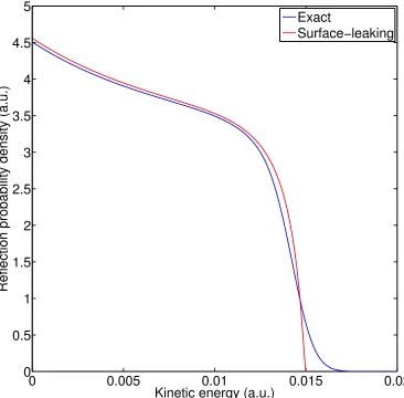
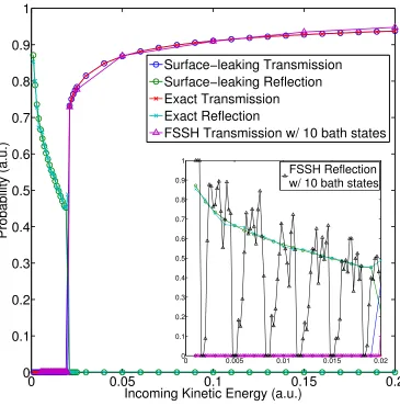
3.2 Model #1: Transmission probability density with large kinetic energy 67 3.3 Model #1: Transmission probability density with small kinetic energy 68 3.4 Model #1: Reflection probability density with small kinetic energy . 69 3.5 Model #1: Surface-leaking and exact transmission and reflection prob-abilities vs. kinetic energy . . . 71

3.6 Model #1: Surface-leaking and exact transmission and reflection prob-abilities vs. coupling strength . . . 72

3.7 Model #3: FSSH, SL-FSSH and exact result of transmission probabil-ity vs. kinetic energy . . . 76

3.8 Model #3: FSSH, SL-FSSH and exact results of transmission proba-bility vs. coupling strength . . . 77

3.9 Model #1: Schematic figure of the dynamics . . . 80

3.10 Model #1: Gaussian averaged transmission probability density with small kinetic energy . . . 81

3.11 Model #1: Transmission probability density with small kinetic energy and different masses . . . 82

4.1 Schematic picture of the Lennard-Jones liquid and electronic hybri-dazation funciton . . . 96 4.2 Cumulative net electron transfer count . . . 107 4.3 The current as a function of the voltage applied . . . 108 4.4 The average number of charged atoms in the system vs. voltage . . . 109 4.5 Normalized distribution of the z coordinates for the positions of the ion 114 4.6 The normalized z-coordinate distribution of the solute atoms during

electron transfer . . . 116 4.7 The normalized z-coordinate distribution of the solute atoms during

electron transfer with larger voltage . . . 117 4.8 The NEMD velocity profiles . . . 121 4.9 I-V curves calculated from NEMD simulations, linear response theory

and a kinetic theory . . . 123 4.10 Cumulative net electron transfer count with different Lennard-Jones

constants . . . 125

5.1 Shifted diabatic harmonic potential energy surfaces and the rates vs. coupling strength . . . 136 5.2 Anharmonic diabatic potential energy surfaces and rates vs. coupling

CHAPTER 1

Introduction

Electron transfer is a ubiquitous process seen in many applications. For instance, in

order to more efficiently harness the solar energy, it is vital for scientists to understand

how excited electrons relax within any solar device: if the excited electrons recombine

quickly with the holes, we cannot harvest any helpful energy other than heat.

Elec-tron transfer also plays a vital role in electrochemistry. The interfacial phenomena in

electrochemistry are dominated by the interplay between molecular dynamics,

elec-tronic interaction and electron transfer, so understanding electron transfer dynamics

is essential for a better understanding of interfacial phenomena.

One straightforward technique to simulate electron transfer is to perform exact

quantum dynamics. However tempting, exact quantum dynamics is feasible only for

very small systems with low dimensionality because the computational cost increases

exponentially. While exact quantum dynamics does not look promising in solving

real-life problems, it does serve as a very useful benchmark of other approximate

techniques, as we will see in the early chapters of this thesis.

To model realistic systems, one attractive category of approximate techniques

is mixed quantum-classical (MQC) methods. In a MQC method, the universe is

separated into two parts – one of them is treated quantum mechanically and the

other classically – so the computational cost can be reduced dramatically while

pre-serving the desired quantum effects. A typical separation treats electrons quantum

mechanically while nuclei classically: the rationale behind this separation is the huge

electron transfer. There are many methods embracing the MQC spirit, including

Meyer-Miller-Stock-Thoss (MMST)/Poisson bracket mapping equation (PBME)1–9_,

multiple spawning10–12 _{and fewest-switches surface hopping (FSSH)}13_{. Among the}

different methods, FSSH is appealing for its simplicity, intuitiveness and high

effi-ciency. Basically, FSSH prescribes that the nuclei are propagated classically on one

of all involved potential energy surfaces (active PES) and the electronic wave

func-tion is propagated according to the Schr¨odinger equation under the instantaneous

nuclear configuration; the electronic transitions dictated by the change of electronic

wave function are modeled by nuclei hoppings between PESs (i.e. changing the active

surface). Thus the nuclear dynamics influence the electronic dynamics through the

instantaneous nuclear configuration, and the electronic dynamics exert feedback on

the nuclear dynamics via induced hops between PESs. In practice, FSSH usually runs

in the adiabatic basis.

We will briefly review the basics of FSSH here. We consider a Hamiltonian in a

diabatic basis:

H=Tn+He (1.1)

whereTnis the nuclear kinetic energy operator andHeis the electronic Hamiltonian.

By diagonalizing He, we obtain the electronic Hamiltonian in adiabatic basis:

He= X

j

Vjj|Φji hΦj| (1.2)

where Vjj is the adiabatic energy (PES) of state j and |Φji is the corresponding

adiabat. We further define the derivative coupling as:

We expand the electronic wave function using the adiabats:

|Ψ(r,R, t)i=X j

cj(t)|Φj(r;R)i (1.4)

Herecj(t) are the time-dependent expansion coefficients. According to the Schr¨odinger

equation, the equation of motion for the coefficients is:

i_~c

.

j

cj

Vij −i~ D

Φi

.

Φj E

= X

j

cj

Vij −i~

.

R·dij

(1.5)

According to FSSH, we make the ansatz that the equation of motion for the nuclei is

simply Newtonian:

dRα

dt =

Pα

Mα (1.6)

dPα

dt =−∇αVλλ(R) (1.7)

Hereα labels a classical degree of freedom and λ is the label for active surface.

Now, let us turn our attention to the hopping probability. We first define the

electronic density matrix element as:

aij ≡cic∗j (1.8)

With this definition, the population on state i is simplyaii while the time derivative

of the population will be:

.

As a sidenote, in the adiabatic basis the first term will be zero as Vij = 0 for i6= j.

The bij can be interpreted as the population reduction on state i that enters state j.

The hopping probability from active stateλ to another state j can be defined as:

gλj = ∆tbjλ

aλλ

(1.10)

∆t is the time step in the simulation. Eq. (1.10) was guessed by Tully13 _{to be the}

hopping probability between adiabatic PESs. Thus, to determine if we need to hop to

another state, we first set all negativegλjto zero. We then compare a random number

ξ (between 0 and 1) to gλj in the following fashion. Assuming λ = 1, if ξ < g12 we

attempt to hop to state 2. If g12 < ξ < g12+g13 we attempt to hop to state 3, etc.

Before we actually change the active surface, however, we need to conserve the energy

of the trajectory by scaling the momentum (assuming that we hop from state λ to

state j):

Pnew =P+ ∆Pdˆλj(R) (1.11)

X

α

(Pα,new)2

2Mα +Vjj(R) = X

α

(Pα)2

2Mα +Vλλ(R) (1.12)

Here ˆdλj(R) is the normalized derivative coupling vector at configuration R. IfPnew

is a complex number, the hop is not energetically feasible so the hop is frustrated

and the active surface remains unchanged. Otherwise the hop is allowed, the active

surface is changed and the momentum is scaled. The premise of rescaling in the

direction of the derivative coupling was first suggested and justified by Herman14–19_,

and later incorporated by Tully13_.

FSSH is not without its issues or limitations. One significant issue is the

when one derives FSSH rigorously20_{. Essentially, FSSH never damps the coherence}

between wavepackets on different PESs, so spurious phenomena appear when two

wavepackets move away from each other. The errors associated with over-coherence

can be consequential given that dephasing and decoherence phenomena for

photo-excited molecules is crucial21,22_{. Previously, many researchers have proposed schemes}

to add decoherence to the FSSH algorithm20,23–38. With this in mind, we will survey

the decoherence issue in chapter 2. However, we will focus on a subject which has

often been neglected, namely the entropy production of surface hopping algorithm.

We find that FSSH cannot conserve the entropy of a closed system, rather the

en-tropy increases when electronic transition occurs. That being said, if we consider

only the electronic subsystem, we find FSSH performs better in recovering the exact

entropy. Nevertheless, in order to reproduce the exact entropy for the model

prob-lems, we show that additional decoherence must be imposed on the FSSH algorithm.

In particular, if we invoke a corrected algorithm – augmented-FSSH (A-FSSH)39,40

– entropic results are greatly improved. Using a frozen Gaussian analysis, we

fur-ther derive an analytical expression for estimating the error in entropy as predicted

by FSSH. This calculation also highlights why, by eliminating the highly oscillatory

coherence when the two wavepackets move apart, A-FSSH improves the stability of

long time dynamics.

In chapter 3, we will investigate another limitation of FSSH. In this chapter, we

focus on the fact that, according to FSSH, electronic states are handled by exact

quantum dynamics, i.e. the Sch¨odinger equation. Just as we have learned from the

story of exact quantum dynamics above, computational cost increases exponentially if

there are a large number of electronic states presented; thus, electron transfer between

than issues of efficiency, frustrated hops in FSSH – which are essential for maintaining

detailed balance – can also lead to artifacts with very many electronic states. To go

beyond standard FSSH, we note that surface-leaking (SL)41 _{was suggested long ago}

to simulate incoherent relaxation into an electronic bath but lacks the capability of

modeling nonadiabatic electronic transitions. The basic idea of surface leaking is that

when an excited molecule couples to a electronic bath, the electron can stochastically

leak into the continuum. When the electron leaks into the continuum, the nuclei will

make a vertical transition to the lower state. Please see Fig. 1.1 for a schematic figure

of the surface-leaking algorithm.

A*-B

A-B

e

-Figure 1.1: Schematic figure of the surface-leaking algorithm. A∗ denotes the excited state of atom (or molecule) A and B is another atom (or molecule) in its ground state. The upper state is coupled to the continuum of states on the right hand side. After the electron leaks into the continuum, the nuclei will make a vertical transition to the lower state.

By incorporating surface-leaking into FSSH, in chapter 3 we propose a new

algo-rithm SL-FSSH that successfully captures the lifetime of the discrete states within the

wide band limit as well as nonadiabatic transitions between discrete states with

rea-sonable accuracy. SL-FSSH is far more efficient than standard FSSH for treating an

marking SL-FSSH, we will find only partial success when going beyond the wide

band approximation. In particular the narrow band limit is captured but the

transi-tion between wide and narrow band is incorrectly predicted. Further study is required

to capture the electronic relaxation beyond the wide band limit.

Now, the SL technique just discussed (chapter 3) is limited to gas phase

phenom-ena. In chapters 4-5, we will study new SH-like techniques for treating molecules near

metal surfaces. While many researchers in electrochemistry focus on the statistical

mechanics of interfacial phenomena, the dynamics of electron transfer between a metal

surface and a molecule nearby can be modeled by a surface hopping (SH) approach

known as a Classical Master Equation (CME)42_{. For such a system, FSSH is not}

fea-sible because of the intractable computational complexity associated with the large

number of states used to model the metal surface. Note here, Shenvi et al.43–45 _have

discretized the continuum of states modeling the metal and run independent-electron

surface hopping (IESH) on the discretized states. While IESH is more efficient than

FSSH, one still has to deal with a large number of states. By contrast, by adopting

an implicit treatment of the continuum of electronic states, the CME does not need

to propagate the wave function as in Eq. (1.5) and the computational complexity is

reduced dramatically. Basically, the probability of electron transfer is dictated by

both the energy difference associated with the change of charge state and the Fermi

level of the metal surface.

Anderson-Holstein model:

H =Hs+Hb+Hc, (1.13a)

Hs=E(x)d†d+V0(x) +

p2

2m, (1.13b)

Hb =

X

k

(k−µ)c

†

kck, (1.13c)

Hc=

X

k

Wk

c†_kd+d†ck

, (1.13d)

d and d† are the annihilation and creation operator for electronic impurity level. ck

and c†_k are the annihilation and creation operator for electronic bath states. µ is the

Fermi level of the electronic bath. If V0(x) is the diabatic PES for the unoccupied

state, we define the diabatic PES for the occupied state to be:

V1(x)≡V0(x) +E(x). (1.14)

The simplest classical master equation can be written as:

∂P0(x, p, t)

∂t =

∂V0(x, p)

∂x

∂P0(x, p, t)

∂p −

p m

∂P0(x, p, t)

∂x

−Γ

~

f(E(x))P0(x, p, t)

+Γ

~(1−f(E(x)))P1(x, p, t), (1.15a)

∂P1(x, p, t)

∂t =

∂V1(x, p)

∂x

∂P1(x, p, t)

∂p −

p m

∂P1(x, p, t)

∂x

+Γ ~

f(E(x))P0(x, p, t)

−Γ

~(1−f(E(x)))P1(x, p, t). (1.15b)

func-coupling between molecule and metal surface. The first two terms in each equation

capture the classical propagation of the population Pi along surfaceVi while the

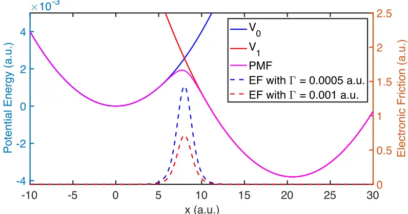
sec-ond two terms dictate the population hopping between two states. In Fig. 1.2, we

plot V0 and V1 for the simplest case: two displaced harmonic oscillators.

In chapter 4, using a very simple molecular dynamics force field combined with

Eq. (1.15), we will simulate the electronic transport through an ionic solution

assum-ing weak electronic couplassum-ing between metal and molecule. Beyond showassum-ing steady

state currents, we will compare nonequilibrium results with those from linear response

theory to demonstrate nonequilibrium effects. These comparisons between

nonequi-librium and equinonequi-librium simulations expand our understanding about how the voltage

and coupling strength move the system away from equilibrium. Furthermore, we build

a kinetic model to reveal the competition between two major processes involved: mass

transport of charge carriers and electron transfer at the electrode surface. The

com-petition is often ignored in simple linear response theories and, by employing the

kinetic model and applying the nonequilibrium velocity profile, we are able to

con-verge linear response results to our nonequilibrium simulation results. In the future, a

more challenging task will be to consider interfacial reactions as well. One easy means

to do so would be to change the force field so as to simulate the trapping of charge

carriers on the electrode surface. However, a more realistic model really requires a

much more sophisticated treatment of electron structure and electron transfer. We

leave this task to the next generation of students.

Finally in chapter 5, we study electron transfer in both the strong and weak

elec-tronic coupling regimes. We will survey and benchmark two different approaches,

namely electronic friction (EF)46 _{and surface hopping (SH/CME)}47_{, using a}

presence of a manifold of electronic states at high temperature using MQC dynamics.

Most research into the AH model has focused on low temperature physics48–59_.

Now, unlike SH/CME dynamics, EF models nuclear dynamics using a potential

of mean force (PMF, Eq. (1.16)) and employs an extra electronic friction (Eq. (1.17))

to model the coupling of nuclear motion to the manifold of electronic states. The

PMF (U(x)) and electronic friction (γe) are defined as

U(x) =V0(x)− 1

β log 1 +e

−βE(x)

. (1.16)

γe= ~

β

Γ f(E(x))(1−f(E(x)))

dE(x)

dx

2

. (1.17)

See Fig. 1.2 for a comparison between diabatic PESs and PMF, and the electronic

friction with small and large electronic coupling. Here, as above, we take the

sim-plest case where V0 and V1 are chosen as dispalced harmonic oscillators. The CME

(Eq. (1.15)) and the EF (Eqs. (1.16)-(1.17)) offer two very different perspectives on

nonadiabatic dynamics. The former should be valid with weak molecule-metal

cou-pling, the latter with strong molecule-metal coupling. Notice that, according to EF

dynamics (Eq. (1.17) and Fig. 1.2), the friction is strongest when the two diabats

cross, such that the electron is constantly hopping back and forth between molecule

and metal.

Surprisingly, in chapter 5, using a shifted harmonic model problem, we find that

EF agrees with the Marcus’s theory even in the nonadiabatic limit. Furthermore,

we find a connection between the Kramer’s theory in the overdamped limit and the

Marcus’s theory, which justifies the correctness of EF dynamics in the nonadiabatic

limit. This hidden connection is perhaps the most exciting result of the present thesis.

from excited dynamics.

Finally, among all the algorithms studied in this thesis, we find a newly proposed

broadened CME (BCME)60,61 _{performs very well in all the cases and we anticipate}

BCME should perform well when describing more realistic systems. According to the

BCME, one effectively runs simulation with SH dynamics on two broadened diabatic

surfaces. See Fig. 5.1(a) in chapter 5.

-10 -5 0 5 10 15 20 25 30

x (a.u.)

-4 -2 0 2 4

Potential Energy (a.u.)

×10-3

0 0.5 1 1.5 2 2.5

Electronic Friction (a.u.)

V₀

V

1

PMF

EF with Γ = 0.0005 a.u. EF with Γ = 0.001 a.u.

Figure 1.2: Diabatic PESs (V0 and V1), PMF (Eq. (1.16)) and electronic friction (Eq. (1.17)) with small (Γ = 0.0005 a.u.) and large (Γ = 0.001 a.u.) electronic coupling.

In the end, this thesis summarizes 4 years of research analyzing how to model

nonadiabatic dynamics both in solution and at a metal surface. Several interesting

results are presented in chapters 2-5. Looking forward, the most interesting question

is how well the BCME performs in a more realistic condensed phase system. Beyond

electron transfer, modeling chemical reactions at metal surfaces in real time is essential

CHAPTER 2

Estimating the Entropy and Quantifying the Impurity of a Swarm of

Surface-Hopping Trajectories: A New Perspective on Decoherence

This chapter is adapted from The Journal of Chemical Physics, Volume 140, Issue

20, Page 204102, 2014.

2.1 Introduction

If the universe is governed by the laws of quantum mechanics and began originally

in a pure state (with zero total entropy), then the universe must always remain in a

pure state thereafter (with zero total entropy). If the universe (with N particles) is

governed by the laws of classical mechanics with density ρ(R, ~~ P ,0) in phase space at

time 0, then the total time-dependent entropy

Scl(t) = Z Z

ρ(R, ~~ P) log(ρ(R, ~~ P)h3N)dR3NdP3N (2.1)

will be conserved throughout time, ∂Scl/∂t = 0. Now both of these predictions do

not match up with the second law of thermodynamics. Starting with Boltzmann’s

celebrated H-theorem62,63 _{there has been a great deal of literature explaining how}

the “effective” entropy of the entire universe tends to grow, provided that one defines

the “effective” entropy as the sum of the entropy of many individual subsystems

(each entangled with their surroundings). These entropic statements hold both for

quantum and classical mechanics. For example, in the case of Boltzmann’s H-theorem

function:

f(R, P) = N

Z

· · ·

Z

ρ(R, R2, . . . R3N, P, P2, . . . P3N)dR2. . . dR3NdP2. . . dP3N (2.2)

SH(t) = Z Z

f(R, P) log(f(R, P)h)dRdP (2.3)

Because the notion of quantum entropy is different from the notion of classical

en-tropy, the question of entropy evolution inevitably arises for mixed quantum-classical

simulations. In particular, for Tully’s fewest switches surface hopping (FSSH)

al-gorithm (which is used extensively nowadays to simulate the dynamics of electronic

relaxation38,64–70_{), one expects interesting questions about entropy to manifest}

them-selves for the FSSH algorithm. After all, by treating quantum electrons separately

from classical nuclei, nuclear-electronic coherence and decoherence can become fuzzy

and counting states (and measuring entropy) may be nontrivial.

To our knowledge, to date there has been no standard definition for the total

entropy of a FSSH calculation, much less a discussion about the role of entropy in

FSSH nonadiabatic dynamics. While many researchers (including the authors) in

the past have focused on “decoherence” corrections to the FSSH algorithm that aim

to fix up the algorithm20,23–38 _{, the total entropy of a FSSH calculation has not}

been quantified previously nor have the origins of irreversibility in FSSH dynamics

been fully explored (though the question of detailed balance has been studied71,72_).

Given the importance of dephasing and decoherence phenomena21,22_{for photo-excited}

molecules (with a system of electrons and a bath of nuclei), we believe a thorough

analysis of surface-hopping entropy is prudent, and the goal of the present paper is

to provide such an analysis in detail.

from the Martens-Kapral mixed quantum classical Liouville equation (QCLE)74–83_{. In}

particular, according to Refs. 20,73, there is a simple prescription for approximating

the partial Wigner transform of the full nuclear-electronic density matrix starting

from a swarm of FSSH trajectories. From such a prescription, we will calculate the

impurity of an FSSH calulation (i.e. one minus the purity) which can serve as an

approximate “FSSH entropy” for systems that are nearly pure.

Finally, armed with a tool to calculate impurity, we will show that total impurity

is not conserved for a closed quantum system propagated by FSSH dynamics. In

other words, even though a pure quantum state in a closed system should remain

pure forever, the impurity of a FSSH calculation increases, as if there is always some

external friction that mixes pure states and moves the system toward equilibrium.

We will examine why impurity increases and how decoherence emerges in the

con-text of partially Wigner transformed wavepackets. Inevitably, our analysis will reach

back to the approximations invoked in Ref. 20. Specifically, according to Ref. 20,

FSSH dynamics will approximate true QCLE dynamics provided that (i) wavepacket

separation is not followed by wavepacket recoherence and (ii) the equation of

mo-tion (EOM) for the off-diagonal electronic density matrix element is modified from

the original time-dependent electronic Schr¨odinger equation. Formally, modifying the

off-diagonal EOM requires a swarm of interacting (rather than independent) FSSH

trajectories, but we have argued that approximations for independent trajectories are

possible (e.g., A-FSSH39,40). Modification of the off-diagonal EOM is necessary to

force the electronic coherences between surfaces 1 and 2 to move along the average

surface – with a force (F1+F2)/2 – as the QCLE stipulates. (This notion of an average

surface has also been discussed by many other authors84–87_{. ) As we will show, the}

An outline of this article is as follows. In Section 2.2, we review the different

definitions of impurity for a Wigner wavepacket moving on one electronic surface. In

Section 2.3, we make a straightforward definition of impurity for a Wigner wavepacket

moving along multiple electronic energy surfaces, and in Sections 2.3.1, 2.3.2, we verify

that this new definition of impurity is conserved by both the Schr¨odinger equation

and the QCLE for a partially Wigner transformed density matrix. In Section 2.3.3,

we define the impurity for a FSSH calculation. In Section 2.4, we present results for

two model Hamiltonians together demonstrating that surface hopping methods do not

conserve the total impurity of the universe. Finally in Section 2.5, we rationalize this

increase in impurity by studying the case of two frozen Gaussians, where an apparently

mixed (i.e. not pure) density matrix arises when one ignores off-diagonal elements

of the partial Wigner density matrix that oscillate rapidly in phase space. In this

sense, decoherence emerges as the result of a stationary phase approximation. For a

seasoned practitioner of surface hopping, who may not be surprised to learn that FSSH

dynamics do not conserve the total impurity of the universe, note that this article

presents a new analytic formulat for estimating FSSH impurity (in Section 2.5.2).

Our notation will be as follows. For indices, i, j, klabel adiabatic electronic states;

M, L, K label joint nuclear-electronic states; α is a general nuclear coordinate; µand

η are indices for a grid point in phase space. For physical quantities, ρ refers to the

full nuclear-electronic density matrix; Φ denotes an adiabatic electronic wavefunction;

Ψ is a joint nuclear-electronic wavefunction; Aij is the partially Wigner transformed

density matrix calculated from surface hopping data; and AW_ij is the exact partially

2.2 Background: The Entropy of a Wigner Wavepacket on One Electronic

Surface

While there are many ways to calculate the quantum entropy88_{, the only approach}

that satisfies all of the Shannon constraints89 _{is the von Neumann entropy:}

S=−Tr(ρlnρ) (2.4)

where ρ is the quantum density matrix. Unfortunately, in practice, calculating the

logarithm in Eq. (2.4) requires diagonalization of the density matrix, which is not

realistic in general for systems with many nuclear degrees of freedom.

For this article, we would like to calculate an approximate entropy of a general

Wigner wavepacket in phase space, which is a subject with a long history88. For one

electronic surface, the Wigner transform is defined by

AW(R, ~~ P , t) = 1 2π_~

Z

d ~Xei ~P·X/~~

*

~ R− X~

2

ρ(t) ~ R+ ~ X 2 + (2.5)

As is well known,AW(R, ~~ P , t) can take on negative values and thus, however

tempt-ing, one cannot simply apply Eq. (2.1) by substituting ρcl(R, ~~ P) = AW(R, ~~ P). Of

course, one could transform to the Husimi distribution, but then the equation of

mo-tion becomes significantly more complicated. As a practical matter, for a Wigner

wavepacket, we require a tractable and easy means to evaluate entropy.

Beyond the von Neumann entropy, a feasible way to estimate the entropy has been

proposed as one minus the purity (impurity)88,90,91_:

S(t) = 1−(2π_~)D Z

d ~Rd ~P

AW(R, ~~ P , t) 2

where D is the number of degrees of freedom. Eq. (2.6) has a number of appealing

properties:

• The impurity is conserved in time according to the time-dependent Schr¨odinger

equation.

• The impurity is 0 for pure states.

• The impurity is positive for mixed states.

Below, we will generalize Eq. (2.6) to the case of many electronic states, and thus

evaluate the impurity of a FSSH calculation. Note that, formally, the defintion of

impurity in Eq. (2.6) is a valid approximation of the von Neumann entropy Eq. (2.4)

only when the universe is close to pure, so that one can expand the density matrix

ρ= 1−z in powers ofz.

2.3 The Impurity of a Partial Wigner Wavepacket on Multiple Electronic

Surfaces

For a physical problem with multiple PESs, the partially Wigner transformed density

matrix is81,82

AW_ij (R, ~~ P , t)≡

1 2π_~

3NZ

d ~Xei ~P·X/~ ~ *

Φi(R~);R~ − X~

2

ρ(t)

Φj(R~);R~ +

~ X

2 +

(2.7)

wheren Φi(

~

R)Eo are the basis of adiabatic electronic wavefunctions at nuclear

is to calculate the impurity as:

S(t) ≡ 1−(2π_~)3N Z

d ~R

Z

d ~P TrAW(R, ~~ P , t)2

= 1−(2π_~)3N X i,j

Z

d ~R

Z

d ~P AW_ij(R, ~~ P , t)·AW_ji(R, ~~ P , t) (2.8)

2.3.1 Exact Dynamics from the Schr¨odinger Equation

To prove that Eq. (2.8) is a meaningful definition of impurity for a system with several

accessible electronic states, we must first prove that, according to this definition,

impurity is conserved in time when a closed system is propagated by the Schr¨odinger

equation. To prove this fact, one starts from a density matrix

ρ=

NK

X

K=1

bK|ΨK(t)i hΨK(t)| (2.9)

In principle,ρcan represent a pure state (NK = 1) or a mixed state (NK >1). The set

{|ΨK(t)i} here denote a basis of orthonormal, fully coupled nuclear-electronic

(2π)3N_{δ(X~), one can calculate the impurity in Eq. (2.8):}

S(t) = 1−(2π_~)−3NX M,L

bMbL Z

d ~P

Z

d ~RX

i,j Z

d ~X

Z

d~Y ei ~P·(X+~ Y~)/~

×

*

Φi(R~);R~ − X~

2

ΨM(t) + *

ΨM(t)

Φj(R~);R~ +

~ X 2 + × *

Φj(R~);R~ −

~ Y 2

ΨL(t) + *

ΨL(t)

Φi(R~);R~ +

~ Y

2 +

= 1−X

M,L

bMbL Z

d ~RX

i,j Z

d ~X

Z

d~Y δ(X~ +Y~)

×

*

Φi(R~);R~ − X~

2

ΨM(t) + *

ΨM(t)

Φj(R~);R~ +

~ X 2 + × *

Φj(R~);R~ −

~ Y 2

ΨL(t) + *

ΨL(t)

Φi(R~);R~ +

~ Y

2 +

= 1−X

M,L

bMbL Z

d ~R

Z

d ~X

× X

i *

Φi(R~);R~ −

~ X 2

ΨM(t) + *

ΨL(t)

Φi(R~);R~ −

~ X 2 + ! × X j *

Φj(R~);R~ +

~ X 2

ΨL(t) + *

ΨM(t)

Φj(R~);R~ +

~ X

2 + !

(2.10)

Now, using the fact that the set of adiabatic electronic eigenstates n Φi(

~

R)Eo is

complete, so that an electronic trace is invariant to the nuclear position associated

with the adiabats,

S(t) = 1−X

M,L

bMbL Z

d ~R

Z

d ~XTre " *

~ R−X~

2

ΨM(t) + *

ΨL(t) ~ R− X~

2 + #

×Tre " * ~ R+ ~ X 2

ΨL(t) + *

where Tre signifies a trace over electronic states. Now, switching variables to

~

ω1 =R~ +

~ X

2 , ~ω2 =

~ R− X~

2, Z

d ~R

Z

d ~X →

Z

d~ω2 Z

d~ω1 (2.12)

we find that the expression for impurity reduces to:

S(t) = 1−X

M,L

bMbLTreTrn

|ΨM(t)i hΨL(t)|

TreTrn

|ΨL(t)i hΨM(t)|

= 1−X

M,L

bMbL|hΨM(t)|ΨL(t)i| 2

= 1−X

M

b2_M (2.13)

where Trn is the trace over nuclei. Thus, in the end, the impurity according to

Eq. (2.8) is clearly time independent and satisfies our intrinsic notation of impurity:

it is zero for pure states and positive for mixed states. Note that, in Eq. (2.13),

S(t) is in fact identical to the fully quantum mechanical impurity, S(t) = 1−Tr(ρ2_).

This agreement between the semiclassical and quantum mechanical impurities arises

only because the impurity in Eq. (2.8) is second order in the density matrix. More

generally, we are unaware of a simple semiclassical formula to estimate even Tr(ρ4)

(much less Tr(ρlnρ)) starting from the Wigner representation.

2.3.2 The Quantum-Classical Liouville Equation (QCLE)

Having proved that the impurity in Eq. (2.8) is conserved according to exact quantum

dynamics, we can show that the impurity of Eq. (2.8) is also conserved in time exactly

is

∂S

∂t = −(2π~)

3NX

i,j Z

d ~R

Z

d ~P

∂ ∂tA

W

ij (R, ~~ P , t)·A W

ji(R, ~~ P , t)

+AW_ij (R, ~~ P , t)· ∂

∂tA

W

ji(R, ~~ P , t)

= −(2π_~)3NX i,j

2 Z

d ~R

Z

d ~PRe

∂ ∂tA

W

ij(R, ~~ P , t)·AWji(R, ~~ P , t)

(2.14)

According to the QCLE, the partially Wigner transformed density matrix evolves

according to

∂ ∂tA

W

ij(R, ~~ P , t) =

−i

~ X

k

VikAWkj −AWikVkj

−X

k,α

Pα

Mα d

α

ikAWkj −AWikdαkj

−X

α

Pα

Mα

∂AW_ij

∂Rα −

1 2

X

k,α

F_ikα∂A

W kj

∂Pα +

∂AW

ik

∂PαF

α kj

!

(2.15)

When we substitute Eq. (2.15) into Eq. (2.14), we find that

∂S

∂t = (2π~)

3N Z ∞

−∞

d ~R

Z ∞

−∞

d ~P Re "

2i

~ X

i,j,k

VikAWkjA W ji −A

W

ikVkjAWji

+ X

i,j,k,α 2Pα

Mα d

α ikA

W kjA

W ji −A

W ikd α kjA W ji +X i,j,α 2Pα

Mα

∂AW

ij

∂Rα A

W ji

+ X

i,j,k,α

F_ikα∂A

W kj

∂Pα A

W ji +

∂AW_ik

∂PαF

α kjA

W ji

!#

= (2π_~)3N Z ∞

−∞

d ~R

Z ∞

−∞

d ~P Re " 2i ~ X i,j

(Vii−Vjj) AW_ij

2

+X

α 2Pα

Mα

X

i,j,k

dα_ikAW_kjAW_ji −X

i,j,k

AW_ikdα_kjAW_ji

!

+X

i,j,α 2Pα

Mα

∂AW_ij

∂RαA

W ji

+X XF_ikα∂A

W kj

∂PαA

W ji +

X∂AW_ik

∂PαF

The first two terms are clearly zero (because there is no real part). Now for the third

and sixth term, by changing the summation index {i, j, k} → {k, i, j}, one finds

∂S

∂t = (2π~)

3N Z ∞

−∞

d ~R

Z ∞

−∞

d ~P Re "

X

α 2Pα

Mα

X

k,i,j

dα_kjAW_jiAW_ik −X

i,j,k

AW_ikdα_kjAW_ji

!

+X

i,j,α 2Pα

Mα

∂AW

ij

∂RαA

W ji + X α X k,i,j

F_kjα∂A

W ji

∂PαA

W ik + X i,j,k ∂AW ik

∂PαF

α kjA

W ji

!#

= (2π_~)3N X i,j,k,α

Z ∞

−∞

d ~R

Z ∞

−∞

d ~P

∂ ∂Rα

Pα

MαA

W ij A W ji + ∂

∂Pα A

W ikF α kjA W ji

= 0 (2.17)

In the last equality, we assume that the density matrix decays to zero sufficiently

fast (as it must for any closed system). Thus, the impurity of a partially transformed

Wigner wavepacket is conserved in time according to the QCLE. This exact

conserva-tion of impurity is somewhat not obvious since the QCLE itself is an approximaconserva-tion

of the quantum Liouville equation. In the future, it might prove interesting to

ex-plore the time evolution of the true von Neumann entropy defined in Eq. (2.4) (rather

than the impurity) according to the QCLE; such an investigation would necessarily

be more complicated than the present article.

2.3.3 FSSH Algorithm and the Calculation of Impurity

Let us now describe how to evaluate Eq. (2.8) with data computed from a surface

hopping simulation. Without loss of generality, we will restrict ourselves to a system

with two electronic states and one spatial dimension. For a typical surface hopping

calculation, one is given a swarm ofNs trajectories, each trajectory carrying an active

surface variableλ= 1,2 (specifying nuclear motion) and a set of electronic amplitudes

A12(R, P, t) are constructed as follows73:

Aii(R, P, t) = 1

Ns X

l

δ(R−Rl(t))δ(P −Pl(t))δ_i,λl_(t) (2.18)

Aij(R, P, t) = 1

Ns X

l

δ(R−Rl(t))δ(P −Pl(t))σ_ijl (2.19)

Here, l is the label for each trajectory andσij is defined as cic∗j. Note that Eq. (2.19)

is not unique (according to Ref. 73) but, in our experience, it has been the most

numerically stable. Finally, we can calculate the impurity with Eq. (2.8) as:

S(t) = 1−2π_~

Z

dR

Z

dP(A11(R, P, t)2+ 2|A12(R, P, t)| 2

+A22(R, P, t)2) (2.20)

In practice, special care must be taken when evaluating the impurity above because

the sum must be evaluated on a finite grid in phase space, with the grid sizes ∆R

and ∆P. Let [Rmin, Rmin+ ∆R, . . . , Rmax −∆R, Rmax] be a grid in position-space,

and [Pmin, Pmin+ ∆P, . . . , Pmax−∆P, Pmax] be a grid in momentum-space. Then, we

evaluate the partial Wigner transform at a grid point (Rµ, Pη) by

Aii(Rµ, Pη, t) = 1 Ns X l Θ ∆R 2 −

Rl(t)−Rµ Θ ∆P 2 −

Pl(t)−Pη

(2.21)

Aij(Rµ, Pη, t) = 1 Ns X l Θ ∆R 2 −

Rl(t)−R_µ Θ ∆P 2 −

Pl(t)−P_η

σ_ijl

(2.22)

where Θ(x) is the Heaviside step function. The impurity is then

S(t) = 1−2π_~X

µ,η

A11(Rµ, Pη, t)2+ 2|A12(Rµ, Pη, t)| 2

+A22(Rµ, Pη, t)2

∆R∆P

one hand, if ∆R and ∆P are too large, the entire wavepacket can be averaged into

one big bin so one does not recover the continuous integral in Eq. (2.20). On the

other hand, if ∆R and ∆P are too small and we do not have enough trajectories,

some bins will contain zero data points because of incomplete sampling, and our final

distribution will appear scattered and distorted. We have done our best to converge

our results to the correct impurity, using 40,000 trajectories.

2.4 Results

To test our approach above, we investigate two standard one-dimensional problems

from Tully’s original paper13_{, the simple avoided crossing and the problem of}

ex-tended coupling. The adiabatic PESs of the two problems are shown in Fig. 2.1. We

study two different variations of surface hopping: 1. Tully’s original fewest-switches

surface hopping (FSSH) and 2. our group’s decoherence-improved augmented fewest

switches surface hopping (A-FSSH) algorithm39,40. The A-FSSH algorithm was

de-signed to build collapsing events on top of FSSH dynamics in order to better simulate

wavepacket separation and decoherence from the perspective of the electronic

subsys-tem following the pioneering work of Prezhdo26_{, Rossky}24,25,32,33_{, Hammes-Schiffer}28_,

Truhlar29–31,34–36 _{and Schwartz}92,93_{. In other words, A-FSSH was designed to better}

estimate the reduced electronic density matrix

σe(t) = Z Z

d ~Rd ~PA(R, ~~ P , t) = 

 

σ11(t) σ12(t)

σ21(t) σ22(t) 



 (2.24)

with corresponding electronic impurity

Se(t) = 1−Tre σe2(t)

−10 −5 0 5 10 −0.02

−0.01 0 0.01 0.02 0.03 0.04

Energy or Energy/distance (a.u.)

r (a.u.) Tully Problem #1 V₁₁(x)

V 22(x) d₁₂(x)/50

−10 −5 0 5 10 −0.25

−0.2 −0.15 −0.1 −0.05 0 0.05 0.1 0.15 0.2

r (a.u.) Tully Problem #3

Energy or Energy/distance (a.u.)

V₁₁(x) V

22(x) d

12(x)

Figure 2.1: The adiabatic PESs for the two standard one-dimensional problems in Tully’s original paper13.

assuming that nuclear wavepackets on different surfaces separate irreversibly.

At time zero, we prepare a Gaussian wavepacket far to the left (x = −15 a.u.)

of the scattering region, starting off on the lower adiabatic PES with width σ = 1

and a momentum of positive 20 a.u.. The particle mass is 2000 a.u.. We transform

to the Wigner representation in phase space to initialize a swarm of surface hopping

trajectories. At a set of different times, we take snapshots of the swarm of trajectories,

digest the corresponding trajectory information into the phase-space grids discussed

above, and then compute the impurity. For reasons of intuition, we also plot the

partial Wigner distribution in phase space for two separate times: (i) right after a

wavepacket is spawned and the wavepackets are still close to the coupling region, and

(ii) at long times, when the wavepackets are already far removed from the coupling

2.4.1 Tully Problem #1: Avoided Crossing

For Tully Problem #1, the electronic Hamiltonian in a diabatic basis is13_:

V11(x) = A[1−exp(−Bx)], x > 0

V11(x) = −A[1−exp(Bx)], x < 0

V22(x) = −V11(x)

V12(x) = V21(x) =Cexp(−Dx2) (2.26)

where A = 0.01, B = 1.6, C = 0.005, and D = 1.0, all in atomic units. See Fig. 2.1

for a picture.

For this problem, the dynamics are simple: a wavepacket enters the coupling

region on the lower adiabat and spawns a new wavefunction on the upper adiabat.

Eventually, two wavepackets emerge from the coupling region – both propagating

forward (in the positive x direction).

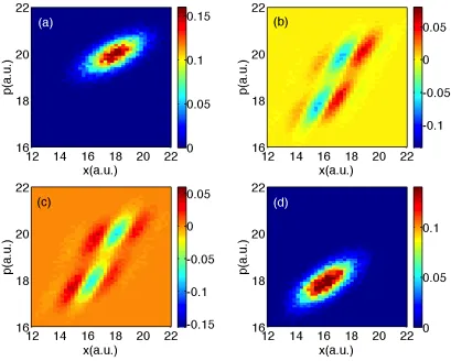
In Figs. 2.2-2.5, we plot the elements of the partially Wigner transformed density

matrix for surface hopping calculations versus exact quantum dynamics. Here, we use

FSSH surface hopping dynamics; note that A-FSSH and FSSH are almost identical

here. The data are plotted at short and long times after the crossing event.

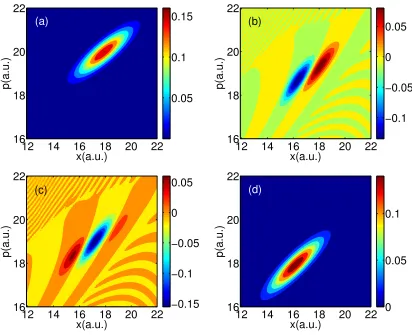
From the data, we see that the FSSH and exact results for the populations AW₁₁

and AW₂₂ agree quite well at all times. However, the FSSH algorithm only partially

recovers the correct form for AW₁₂. Whereas exact quantum dynamics predicts only

two peaks (one positive, the other negative) for the coherence, FSSH predicts multiple

peaks that are correlated with the diagonal peaks. The agreement gets worse for long

times. According to exact quantum dynamics, there are also small oscillations in

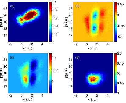
Figure 2.2: FSSH data for Tully #1. The densities are plotted in phase space at time 1590 a.u., (a) top-left A11; (b) top-right Re(A12); (c) bottom-left Im(A12); and (d) bottom-rightA22.

x(a.u.)

p(a.u.)

−2 0 2 4

17 18 19 20 21 0.0 0.02 0.04 0.06 0.08 0.1 x(a.u.) p(a.u.)

−2 0 2 4

17 18 19 20 21 −0.1 −0.05 0 0.05 x(a.u.) p(a.u.)

−2 0 2 4

17 18 19 20 21 0 0.05 0.1 0.15 0.2 x(a.u.) p(a.u.)

−2 0 2 4

17 18 19 20 21 0 0.05 0.1 (a) (c) (b) (d)

x(a.u.)

p(a.u.)

12 14 16 18 20 22 16 18 20 22 0.05 0.1 0.15 x(a.u.) p(a.u.)

12 14 16 18 20 22 16 18 20 22 −0.1 −0.05 0 0.05 x(a.u.) p(a.u.)

12 14 16 18 20 22 16 18 20 22 0 0.05 0.1 x(a.u.) p(a.u.)

12 14 16 18 20 22 16 18 20 22 −0.15 −0.1 −0.05 0 0.05 (a) (c) (b) (d)

2.4.2 Tully Problem #3: Extended Couplings

For Tully problem #3, the electronic Hamiltonian in a diabatic basis is13_:

V11(x) = −A

V22(x) = A

V12(x) = Bexp(Cx), x < 0

V12(x) = B[2−exp(−Cx)], x >0 (2.27)

whereA = 0.0006, B = 0.1 andC= 0.9, all in atomic units. See Fig. 2.1 for a picture.

For this model Hamiltonian, the dynamics are more complicated than the previous

problem. Here, one wavepacket begins far to the left on the lower adiabat and, moving

to the right, a second wavepacket is spawned on the upper adiabat. Afterwards, the

two wavepackets continue moving right and leave the coupling region. At time 1650

a.u., the wavepacket on the lower adiabat is moving quickly to the right and eventually

it will transmit with nearly 100% probability. At the same time, the wavepacket on

the upper adiabat has slowed down and is in the process of turning around; this

wavepacket will reflect with nearly 100% probability. Later on, before time t= 3300

a.u., the reflecting wavepacket on the upper adiabat will spawn another wavepacket

on the lower adiabat, and both of these wavepackets will then move together to the

left asymptotically.

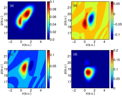
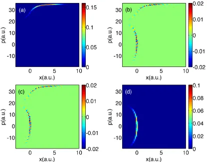
In Figs. 2.6-2.8, we plot results for A-FSSH, FSSH and exact quantum dynamics at

time 1650 a.u., not long after the spawning event. Note that the population data from

FSSH and A-FSSH track the exact quantum dynamics data nearly quantitatively.

coherence matrix element is centered midway between the AW

11 and AW22 population

matrix elements. By contrast, FSSH predicts that the coherences should be centered

on the population peak positions (just as for Tully problem #1). At the same time,

because of a collapsing event triggered by wavepacket separation, A-FSSH predicts

almost exactly zero coherence.

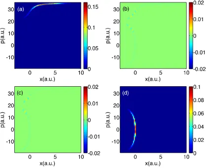
Finally, for long times (t = 3300 a.u.), we plot all data in Figs. 2.9-2.11. Focusing

first on populations, exact quantum dynamics reveals a small peak in between the two

centers of populations around (x, p) ≈ (5,5); this feature is absent from the surface

hopping data and will be explained in Section 2.5.1. Otherwise, the surface hopping

data looks qualitatively correct.

With regards to the coherences in Figs. 2.9-2.11, exact quantum dynamics

pre-dicts that the off-diagonal matrix element is incredibly small except for a small peak

midway between the two population centers at (x, p) ≈(5,5) and phase oscillations

are observed around that peak. Neither A-FSSH nor FSSH find such a peak nor such

oscillations; these features will also be explained below.

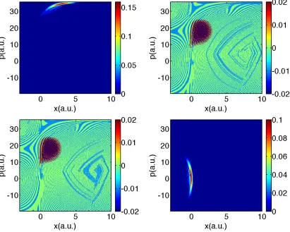
Interestingly, notice that, if one looks at A12 in Fig. 2.9 around the transmitting

peak at (x, p) = (30,45), the FSSH decoherence problem is barely visible. In fact, the

FSSH coherence density appears almost as small as the A-FSSH coherence density,

even though we know that, for this specific problem, the FSSH methodology breaks

down26,92_{; unlike A-FSSH, the FSSH algorithm fails to account for the bifurcation}

between transmitting and reflecting wavefunctions. To explain this surprising feature,

recall that, for these figures, we are averaging over finite chunks of phase space; as

we have explained in Ref. 94, Tully problem #3 is pathological because, by chance,

averaging removes FSSH’s decoherence problems. To prove that the FSSH coherences

Figure 2.6: FSSH data for Tully #3: Time is 1650 a.u.. Same notation as in Fig. 2.2.

cancellation of sign, in Fig. 2.12 we plot the function:

Anorm₁₂ (R, P, t)≡ 1

Ns X

l

δ(R−Rl(t))δ(P −Pl(t))σ_ijl

(2.28)

From Fig. 2.12, it is clear that each FSSH trajectory carries an electronic density

matrix with a large off-diagonal component, and the FSSH algorithm does well only

because averaging over a phase space volume allows for a fortuitous sign

p(a.u.)

−10

0

10

20

30

−20

−10

0

10

20

30

0

0.02

0.04

0.06

0.08

p(a.u.)

x(a.u.)

−10

0

10

20

30

−20

−10

0

10

20

30

0

0.02

0.04

0.06

0.08

(a)

(b)

2.4.3 Impurity

Having analyzed the capacity of surface hopping methods to recover the partial

Wigner transform densities in phase space, in Fig. 2.13 we plot the total impurity

(S(t), Eq. (2.20)) as function of time both for FSSH and A-FSSH trajectories. Here,

∆Rand ∆P are chosen by insisting that the total impurity be zero at time zero, and

we have checked that our data are changed only slightly by altering the grid sizes.

According to Fig. 2.13, we find that the total impurity grows in time for both

FSSH and A-FSSH as soon as particles start hopping in between surfaces. As we will

show in Section 2.5.2, one can evaluate this growth in total impurity analytically for

simple problems (e.g., for Tully #1). From the data in Sections 2.4.1 and 2.4.2, it is

clear that this growth in total impurity can be attributed to the off-diagonal errors

of FSSH.

Interestingly, according to Fig. 2.13, even though A-FSSH incorporates

decoher-ence, FSSH and A-FSSH yield very similar total impurities. This coincidence can be

explained by the simple fact that neither algorithm captures the exact coherence and

neither can correctly recover recoherences. The premise of the A-FSSH algorithm is

that, since recoherences cannot be captured correctly by any Tully-style surface

hop-ping algorithm, one should damp the electronic coherences after wavepackets separate

so that long time dynamics (without recoherences) will be stable and accurate95. In

other words, A-FSSH was designed to recover the correct impurity of the electronic

subsystem (which is entangled with the nuclei).

To prove that A-FSSH delivers on this promise, we plot the elements of reduced

electronic density matrix and electronic impurity (Se(t), Eq. (2.25)) in Figs. 2.14-2.15.

From the figures, we observe that A-FSSH recovers qualitatively the exact reduced

0 500 1000 1500 2000 2500 3000 0

0.1 0.2 0.3 0.4 0.5

Time(a.u.)

Total Impurity

Tully#3 FSSH Tully#3 AFSSH Tully#1 FSSH Tully#1 AFSSH

Tully#1 4|c₁|4|c₂|4

Figure 2.13: The total impurity S(t) from Eq. (2.20) for the FSSH and A-FSSH algorithms for Tully problems #1 and #3. We also plot Eq. (2.42), an approximate analytical result for frozen Gaussians. The total impurity of the exact quantum system is zero for all time.

electronic density matrix for Tully problem #3. Moreover, in both cases, A-FSSH

exactly reproduces the impurity of the electronic subsystem (which grows in time as

would be expected). Note that FSSH recovers neither the correct reduced electronic

0 1000 2000 3000 0.4 0.6 0.8 1 1.2 1.4 Time(a.u.) σ1 1 FSSH A−FSSH Exact

0 1000 2000 3000 −0.1 0 0.1 0.2 Time(a.u.) R e( σ1 2 ) FSSH A−FSSH Exact

0 1000 2000 3000 −0.2 −0.1 0 0.1 0.2 0.3 Time(a.u.) Im ( σ1 2 ) FSSH A−FSSH Exact

0 1000 2000 3000 −0.2 0 0.2 0.4 0.6 Time(a.u.) Electronic Impurity FSSH A−FSSH Exact (a) (b) (c) (d)

0 1000 2000 3000 0.4 0.6 0.8 1 1.2 1.4 Time(a.u.) σ 1 1 FSSH A−FSSH Exact

0 1000 2000 3000 −0.4 −0.3 −0.2 −0.1 0 0.1 Time(a.u.) R e ( σ1 2 ) FSSH A−FSSH Exact

0 1000 2000 3000 −0.1 0 0.1 0.2 0.3 0.4 Time(a.u.) Im ( σ1 2 ) FSSH A−FSSH Exact

0 1000 2000 3000 −0.2 0 0.2 0.4 0.6 Time(a.u.) Electronic Impurity FSSH A−FSSH Exact (a) (b) (c) (d)

2.5 Discussion: Frozen Gaussian Dynamics in a Partially Transformed

Wigner Phase Space

2.5.1 Exact Quantum Dynamics Predicts Nonlocal Coherences and Phase

Oscillations

The data in Sections 2.4.1 and 2.4.2 highlighted the fact the surface hopping dynamics

can recover the populations well (compared to the exact partial Wigner transform),

but off-diagonal coherences are not as accurate. These results should not be very

sur-prising to a reader familiar with Ref. 20, where it was shown that (i) the on-diagonal

equations of motion for FSSH are almost exactly the same as the corresponding QCLE

equations of motion; but (ii) the off-diagonal equations of motion for FSSH need a

severe correction to approximate the corresponding QCLE equations of motion. And

formally, these corrections require interacting (rather than independent) trajectories.

In the present manuscript, we have seen that the FSSH errors in off-diagonal

coher-ence lead effectively to a growth in total impurity over time.

To better interpret our data from Sections 2.4.1 and 2.4.2, we will now find it

useful to investigate wavepacket bifurcation in phase space from the perspective of

frozen Gaussian nonadiabatic dynamics. With a frozen Gaussian ansatz, the total

nuclear-electronic wavefunction has the following form20:

Ψ(~r, ~R, t) =c1g(R~;R~1(t), ~P1(t))Φ1(~r;R~) +c2g(R~;R~2(t), ~P2(t))Φ2(~r;R~) (2.29)

where g represents a nuclear Gaussian wavepacket

g(R~;R~s(t), ~Ps(t)) ≡ Y

α

1

πa2 Rα

1/4 exp

₋

(Rα_−Rα s(t))2 2a2

Rα

According to Eq. (2.7), the partial Wigner transform for a frozen Gaussian is (for

i= 1,2)

AW₁₁(R, ~~ P) = |c1| 2

(π_~)3N Y

α exp

−(Rα−Rα₁)2

a2 Rα

exp

−(Pα−P₁α)2a2_Rα

~2

(2.31)

AW₂₂(R, ~~ P) = |c2| 2

(π_~)3N Y

α exp

−(Rα−Rα₂)2

a2 Rα

exp

−(Pα−P₂α)2a2_Rα

~2

(2.32)

AW₁₂(R, ~~ P) = c1c

∗

2 (π_~)3N

Y

α exp

_−(Rα₋1 2(R

α

1 +Rα2))2

a2 Rα

×exp

₋

(Pα− 1 2(P

α

1 +P2α))2a2Rα

~2

exp

i(R₂α−Rα₁)Pα

~

×exp

i(P₁α−P₂α)Rα

~

exp

i(P₂α−P₁α)(Rα₂ +Rα₁) 2_~

(2.33)

By integrating the squares of Eqs. (2.31)-(2.32) and plugging into Eq. (2.20), it is

straightforward to prove (as it must be) that the impurity of a frozen Gaussian ansatz

is always zero, S = 0.

Two key observations emerge from Eqs. (2.31)-(2.33):

1. According to exact quantum dynamics, the off-diagonal coherence matrix

ele-mentAW₁₂ should pick up a phase that oscillates very quickly throughout phase

space, proportional to (R~1 −R~2) and (P~1 −P~2).

2. According to exact quantum dynamics, the off-diagonal coherence density in

phase space is not centered at the same location as the on-diagonal population

densities. In particular, the off-diagonal coherence density matrix is centered

at (R~1+R~2)/2,(P~1+P~2)/2

.

qual-2.11. The nonlocality of the AW

12 density in phase space is also completely consistent

with the QCLE which postulates that, to first order in _~, AW

12 coherences should be

propagated with forces (F~1+F~2)/2 [while the populations AW11 (AW22) are propagated,

of course, alongF~1 (F~2)].

As a sidenote, we mention that, even for a wavefunction with two frozen Gaussians

onthe same electronic surface AW₁₁ – the first wavepacket centered at (R~(a)₁ , ~P(a)₁ ) and

the second wavepacket centered at (R~(b)₁ , ~P(b)₁ ) – one still finds a nonlocal peak in the

Wigner transform centered at (R~(a)₁ +R~(b)₁ )/2 and (P~(a)₁ +P~(b)₁ )/2. These nonlocal

peaks are a well-known feature of Wigner transforms96_{, and this explains the peak in}

the middle of Fig. 2.11(a).

Overall, partially Wigner transformed density matrices can produce complicated,

nonlocal phase space densities.

2.5.2 FSSH Predicts Local Coherences: An Analytical Measure of FSSH

Impurity

Let us now consider frozen Gaussian dynamics from the perspective of the FSSH and

A-FSSH algorithms, and calculate our definition of impurity. To simplify the notation,

we define f1(R, ~~ P) and f2(R, ~~ P) as the normalized nuclear densities in phase space

for adiabats 1 and 2 (for i= 1,2):

fi(R, ~~ P) = 1 (π_~)3N

Y

α exp

₋

(Rα_−Rα i)2

a2 Rα

exp

₋

(Pα_−Pα i )2a2Rα

~2

, (2.34)

For the FSSH algorithm, the diagonal elements of the partially Wigner transformed

density matrix are then (for i= 1,2)