A statistical model to estimate the local vulnerability to severe weather

(1)

https://doi.org/10.5194/nhess-18-1617-2018 © Author(s) 2018. This work is distributed under the Creative Commons Attribution 4.0 License.

A statistical model to estimate the local vulnerability

to severe weather

Tobias Pardowitz1,2

1_{Optimal Use of Weather Forecast Branch, Hans Ertel Centre for Weather Research, Germany}

2_{Institute of Meteorology, Freie Universität Berlin, Carl-Heinrich-Becker Weg 6–10, 12165 Berlin, Germany}

Correspondence:Tobias Pardowitz ([email protected]) Received: 8 September 2017 – Discussion started: 12 September 2017 Revised: 27 April 2018 – Accepted: 3 May 2018 – Published: 13 June 2018

Abstract. We present a spatial analysis of weather-related fire brigade operations in Berlin. By comparing operation oc-currences to insured losses for a set of severe weather events we demonstrate the representativeness and usefulness of such data in the analysis of weather impacts on local scales. We investigate factors influencing the local rate of operation oc-currence. While depending on multiple factors – which are often not available – we focus on publicly available quanti-ties. These include topographic features, land use informa-tion based on satellite data and informainforma-tion on urban struc-ture based on data from the OpenStreetMap project. After identifying suitable predictors such as housing coverage or local density of the road network we set up a statistical model to be able to predict the average occurrence frequency of lo-cal fire brigade operations. Such model can be used to deter-mine potential “hotspots” for weather impacts even in areas or cities where no systematic records are available and can thus serve as a basis for a broad range of tools or applica-tions in emergency management and planning.

1 Introduction

It has been stated within the Sendai Framework for Disaster Risk Reduction 2015–2030 by the United Nations (UNISDR, 2015) that the implementation of effective disaster risk re-duction measures should be based on an understanding of disaster risks, including all its dimensions of vulnerability, capacity, exposure of persons and assets, hazard characteris-tics and the environment. On local and national levels, this requires to systematically evaluate, record, share and pub-licly account for disaster losses to gain understanding of the

impacts in the context of event-specific hazard, exposure and vulnerability information.

While insurance records are a very useful data source and have been used in many analyses of regional weather im-pacts, their availability is generally limited due to economic interests of insurance providers. Making use of records of lo-cal emergency managers (first responders) yields an immense potential as an alternative database for analysing weather im-pacts, particularly on local scales. While often such records exist, they mostly lack systematic and homogenous data for-mat and quality standards. Definition of such data standards must be regarded key requisite to be able to scientifically ad-dress disaster losses as required within the Sendai Frame-work.

(2)

fore-cast data can in fact improve forefore-casts of daily ambulance demand (Wong and Lai, 2014).

There have been only few studies making use of spatial information of emergency operation data (i.e. the location of an assistance request) in relation to severe weather events. Two studies by Schuster et al. (2005) and Rossi et al. (2013) compared emergency call data with radar reflectivity data for a severe hailstorm event and found a satisfying representa-tion of the hailstorm path in the density of emergency calls on the ground. Other studies have tried to utilize similar data, but they faced problems concerning the availability of accu-rate data. As described in Busch (2008), problems can occur in the case of catastrophic events since the archiving of fire brigade operation data is often limited in such cases. In par-ticular, this means that spatial information on the individual location of operations is not archived, hindering spatial anal-yses for these events.

Pardowitz and Göber (2016) have demonstrated – similar to the studies mentioned above – that satisfying correspon-dence of radar reflectivity for severe thunderstorm events and locations with occurrences of fire brigade operations can be found. However, this occurrence is strongly modulated by other factors such as the density of buildings. This is a con-firmation of the common understanding that the occurrence and height of impacts are determined by the simultaneous existence of a hazard and vulnerability against this hazard.

Approaches to address the local vulnerability have been developed in flood impact modelling. Apel et al. (2009) and Jongman et al. (2012) describe different modelling ap-proaches to estimate economic damages for flood events (particularly the 2002 flood event in Saxony). Based on data from digital elevation models (DEMs), local damages are estimated in dependence of inundation depth. Furthermore, such depth–damage relation can be differentiated – e.g. by considering information on land use – to account for variable vulnerabilities.

In this study we focus exclusively on the estimation of predictors describing the local vulnerability and exposure. We thus neglect temporal variations of weather parameters and investigate the long-term averaged occurrence frequen-cies (which can be regarded as the equivalent to a local “cli-matology”) of fire brigade operations. We also test whether it is possible to predict these long-term occurrence frequen-cies for areas in which we might not have actual operation records available.

Based on a new data set of fire brigade operations in Berlin for the period of 2002–2012, this study aims at assessing the latter, namely the vulnerability against hydrometeorological hazards. In a first step we analyse this new data set particu-larly with respect to the question of how these impacts are re-lated to building damages induced by windstorms and thun-derstorms. It needs to be noted that neither insurance loss data nor the archive of fire brigade operation extensively de-scribes all possible weather impacts. Instead it is important to investigate the different causes of weather impacts included

in the individual data sets. Within the metropolitan area of Berlin, we then aim to identify factors describing the local vulnerability and thus influencing the local risk for weather impacts as given by the fire brigade operations. Potential fac-tors include topographic features, land use information based on satellite data and information on urban structure based on data from the OpenStreetMap (OSM) project. After identify-ing suitable predictors such as housidentify-ing density or local den-sity of the road network we set up a statistical model to be able to predict local operation densities. Such model can be used to determine potential “hotspots” for weather impacts even in areas or cities where no systematic records are avail-able.

The remainder of this paper is structured as follows. Sec-tion 2 describes the various data sets that are used to de-scribe impacts as well as potential predictors for vulnerabil-ity. Methodological steps and modelling approaches are de-scribed in Sect. 3, while results are shown in Sect. 4. Finally, Sect. 5 provides a discussion of results as well as the major conclusions that can be drawn from this study.

2 Data

2.1 Fire brigade operations

(3)

op-Table 1.Distributions of impacts of different types in Berlin for the period 2002–2011, stratified by their cause and by season, i.e. winter and summer half year and temporal correlations to daily building damages.

Full year Summer Winter

Absolute Total Correlation Summer Correlation Winter Correlation with number fraction with daily losses share with daily losses share daily losses

All operations 10.069 100 % 0.58∗∗∗ 50 % 0.59∗∗∗ 50 % 0.57∗∗∗

Water damage 3.358 33 % 0.14∗∗∗ 53 % 0.06 47 % 0.41∗∗∗

Traffic obstruction 2.549 25 % 0.22∗∗∗ 46 % 0.15∗∗∗ 54 % 0.30∗∗∗

Tree-related 1.715 17 % 0.67∗∗∗ 73 % 0.69∗∗∗ 27 % 0.74∗∗∗

Construction element 1.407 14 % 0.58∗∗∗ 45 % 0.59∗∗∗ 55 % 0.67∗∗∗

Ice and snow 211 2 % 0.00 0 % − 100 % 0.00

Others 831 8 % 0.00 18 % 0.01 82 % 0.01

Significance is indicated ifpvalue is below 0.05 (∗_{), below 0.01 (}∗∗_{) and below 0.001 (}∗∗∗_).

erations (about 7500 per year) accounted for about 20 % of all operations. Note that ambulance call outs (∼245 000 per year) and false alarms (∼31 000 per year) have been disre-garded here. Most weather-related operations are due to wa-ter damages (33 %). Traffic obstruction accounted for 25 % of operations and tree-related operations for about 17 % (Ta-ble 1). Operations related to construction elements accounted for about 14 % and ice- and snow-related operations for 2 %. Some other keywords (individually accounting for 1 % or less each) were used, which sum up to about 8 %. Stratify-ing by season shows that, in total, operations are equally dis-tributed over winter (October–March) and summer half year (April–September). This choice is done primarily to best dis-criminate between thunderstorm and winter storm impacts (see e.g. Donat et al., 2011). The individual types of oper-ations, however, partly show distinct differences in summer and winter (Table 1). Particularly tree-related operations oc-cur mainly in summer (73 %) while ice- and snow-related operations naturally occur in winter exclusively.

2.2 Building loss data

Insurance data on windstorm and thunderstorm losses to residential buildings were provided by the German in-surance association (Gesamtverband der Deutschen Ver-sicherungswirtschaft e.V., GDV). Berlin-wide damages are available on a daily basis for the period 1997–2011, while data at the zip code level (190 within Berlin) are available for a small selection of events only. Direct (liquid) precipi-tation damages as well as flooding damages are not part of the available data set even though they might be highly rel-evant in the case of severe precipitation related to thunder-storm events. Still, for investigations of severe weather events – particularly small-scale events such as thunderstorms – in-surance loss data are thus extremely valuable. However, dif-ficulties arise when interpreting the insurance data since the data set does not allow a direct attribution of losses to their cause (i.e. hail or windstorm induced). In addition, faulty

at-tribution of individual insurance claims (both temporal and spatial) can cause inaccurate loss figures. For example, this can be because the exact day of occurrence of a damage is unknown in some cases. In addition, if damage occurs at a house managed by a real estate company, the insurance claim might be attributed according to their administrative centre instead of the actual origin. For the set of events for which insured loss data are available on zip code area, an evaluation of the spatial patterns and a comparison to the occurrences of fire brigade operations can be made. The selection of events contains the four windstorm events with the highest impacts in Berlin within the reference period 2007–2011 (Kyrill on 17–19 January 2007, Lothar07 on 24–28 May 2007, Emma on 28 February–2 March 2008, Xynthia on 27 February–1 March 2011) and two convective events (Aram on 6 June 2011 and Gunnar on 22 June 2011), which have been selected because they were studied in detail in Wapler et al. (2015). The data set comprises area-wide coverage of losses due to windstorm and thunderstorm. Also, to address the temporal correlation of different impacts, Berlin-wide losses are anal-ysed and compared to total operation counts within Berlin. According to the insurance loss records (covering windstorm and hail damages), EUR 8.12 Mio in damage is recorded for Berlin per year. The temporal distribution is rather balanced with 48 % of damage occurring in summer and 52 % in win-ter. While most damage in winter is related to intense winter windstorms (Klawa and Ulbrich, 2003; Pinto et al, 2010; Do-nat et al., 2011), a large share of summer damage is due to thunderstorms and in particular due to hailfall (Aller and Ko-zlowski, 2008; Kunz and Puskeiler, 2010).

2.3 OpenStreetMap data

(4)

on road networks. As a first predictor, the number of build-ings per grid cell on a regular 1×1 km grid is derived. Also, by including information on housing extent, the fraction of the grid cell covered by buildings is calculated. As discussed later, even though these quantities are highly correlated, both predictors should be considered to distinguish between the high-density city centre with very large buildings and suburban areas with large numbers of detached houses. Additionally, the density of the road networks is considered by calculating the total length of road segments within a 1×1 km grid cell (specified as a length per grid cell area, thus km km−2). The OSM data set contains a classification of the road networks (the major categories being highway, primary, secondary and tertiary road networks), which is why road densities can be assessed individually for these classes. It would be valuable to add the population density as a predictor as well. However, population density is not freely available on the spatial resolution required in this analysis (1 km). Freely available data sets include the CIESIN global gridded data set (with a resolution of about 5 km) or that of the German Federal Statistical Office (DESTATIS), which is available on a district level only.

2.4 CORINE land cover data

The CORINE (Coordination of Information on the Environ-ment) land cover (CLC) data set provides European-wide in-formation on land cover and land use, based on a unified clas-sification of the most important types of land usage (CEC, 1994; Bossard et al., 2000, Büttner et al., 2012). More specif-ically, we used CLC2006, which is based on SPOT-4/5 and IRS P6 LISS III satellite data. Geometric accuracy of satel-lite images is specified to be smaller than 25 m and result-ing minimum mappresult-ing units within CLC are specified to be 25 ha, with the geometric accuracy of the CLC data being better than 100 m. In total, 44 land usage classes are used in CLC2006 as subcategories of the main land usage types: “artificial surfaces”, “agricultural areas”, “forest and semi-natural areas”, “wetlands” and “water bodies”. More details on CLC2006 can be found in Büttner et al. (2012). The orig-inal data consist of polygon data in the form of shape files, which have been processed to calculate land use characteris-tics on a grid-point basis. For this, the area fractions of all 44 CLC types (adding up to 100 %) are calculated on a speci-fied grid. Here we use a regular long–lat grid with a 1×1 km resolution. These gridded fields of the area fraction are then used as predictors in the following analyses.

2.5 Data from DEM

Data from the digital elevation model dgm200 (GeoBasis-DE/BKG 2016) are also used to derive orographic height and slope. Original data have a horizontal resolution of 200 m and are available for Germany. Alternatively, GTOPO30 has been used, which has a lower horizontal resolution

of 30 arcsec (approximately 1 km). However, GTOPO30 is available globally. The data are used to derive orographic height as well as the slope on a regular 1×1 km grid for Germany. In the case of dgm200, which has a finer resolution compared to the target grid, orographic height is calculated as the average height over all original 200 m×200 m grid boxes within a target grid box. In the case of GTOPO30 orographic height on the target grid is determined by means of a nearest neighbour remapping. Since differences for the Berlin region were negligible, dgm200 has been used in the following. The slope is calculated according to the algorithm proposed by Horn (1981). The algorithm also assesses the aspect, which – in further studies – might be considered as an additional vulnerability predictor. However, since the area for which the vulnerabilities are analysed is limited to Berlin (featur-ing no considerable height variations), topographic features play only a minor role here. However, in future studies in-cluding other investigation areas, topographic features may be more important to consider.

3 Methodology

3.1 Comparison of fire brigade operations and building damage data

To assess how representative spatial information on weather impacts on a sub-city scale can be derived from the data set and whether there is a temporal correspondence be-tween daily damages and operation numbers, a comparison of building loss data and fire brigade operations is performed. While insured losses on residential housing comprise spe-cific impacts caused by windstorms and thunderstorms, fire brigade operations can be caused by additionally meteoro-logical phenomena such as flooding (which is not included in the loss data set) or impacts due to freezing rain or road icing. The aim of this comparison is to identify how specific categories of fire brigade operations (i.e. tree-related opera-tions) are related to the wind and hail impacts as described by the insured loss data. It can be expected that other cate-gories (operations due to road icing) will not relate to insured losses.

(5)

dif-ference in results was tested using the Spearman rank corre-lation. It was found that results are not qualitatively affected by the chosen correlation method. Correlations are tested for significance by testing whether the Pearson’s product mo-ment correlation follows at distribution. Significance of cor-relations is assessed by considering the resulting p values. Daily total operation counts for Berlin are furthermore com-pared to Berlin-wide damages, which are available on a daily level for the period of 2002–2011. Temporal correlations to daily building damages are calculated, again for both total count and counts for operations related to individual key-words.

3.2 Spatial correlation between potential vulnerability predictors and patterns of operation occurrences To identify predictors for vulnerability, a spatial correlation analysis between numerous quantities derived from the dif-ferent geospatial data sets and gridded operation densities is performed. Variables include gridded densities of man-made structures (buildings, streets), topographic features (height, slope) and land use information. The latter is pre-processed such that the area fraction of a specific land use type (as spec-ified in the CORINE data set) within each 1×1 km grid box is given. Again, spatial correlations are assessed using either operations of one specific category or operations irrespec-tive of their type. As described above, correlations are calcu-lated using the Pearson correlation. Again, using the Spear-man rank correlation did not qualitatively affect the results. Significance of correlations is assessed as described in the previous section.

3.3 Multiple linear regression model

On the basis of the set of potential vulnerability predictors (as listed in Table 3), a statistical model is set up based on multiple linear regression to analyse the predictability of the spatial distribution of (long-term) operation occurrence rates. Such model could potentially be used to identify “hotspots” in the local occurrence of operations in areas where no ex-plicit data on operations are available and might be highly relevant in terms of long-term planning of capacities for ef-fective emergency management. In the following, three dif-ferent types of models are addressed. A linear model, a log-arithmic variant (assuming a log-normal distribution of the predictant, modelling the logarithm of operation density) and a Poisson model (typically used to model count variables). To provide robust results and prevent overfitting of the data, an appropriate subset of variables must be chosen from the set of available predictors. This is particularly important since some predictors are highly correlated amongst each other, which is referred to as multicollinearity (Belsley et al. 1980). Even though multicollinearity does not reduce the predictive power of the model, it may strongly affect the interpretation of individual regression coefficients of predictors containing

mutual information. Besides being the cause of overfitting, it is thus desirable to reduce the number of (correlated) predic-tors to also better interpret resulting regression coefficients. To do so we chose an iterative procedure which – starting from an initial model – stepwise removes or adds predictor variables. Which predictor to add to (or remove from) the list of predictors in the model is decided in each iterative step by maximization of the Akaike information criterion (AIC; see Akaike, 1985). The basic idea is to assume a certain penalty for each (additional) predictor within the model. This penalty needs to be balanced to the resulting goodness of the model fit (e.g. by means ofR2), leading to an optimization prob-lem between the total penalty and fit quality. The algorithm converges if no predictor can be added or removed to further optimize the model in terms of the AIC. To perform this op-timization procedure, the weight of the penalty can be varied by means of the parameterk. Whilek=2 corresponds to the classical AIC, higherkresult in an increased penalty for ad-ditional predictors. Different choices ofkwill ultimately lead to different optimized models including more (less) predictor variables ifkis lower (higher).

3.4 Model validation methodology

To assess the predictive skill of the optimized model a cross validation is set up. For this, the area of Berlin is divided into four sectors. Then the model – using the set of predic-tors identified by means of the iterative procedure described above – is fitted four times, each time using all grid points within three of the four sectors. Each model fit is then used for predicting the operation density for grid points within the fourth sector. In this way predictions are obtained for data that have not been used for model fitting. Calculating the mean square error of these model predictions in compari-son to observed operation density values results in the cross-validation error, which is used as the criterion for predictive model skill. The optimal choice of k in the iterative opti-mization procedure described above is not known up front. Different choices ofklead to differing numbers of predictor variables. Thus, to find the optimal model for predictive pur-poses, we varyk and compare the predictive model skill of the resulting models. The optimal choice is found by maxi-mizing the predictive model skill, i.e. minimaxi-mizing the cross-validation error.

4 Results

4.1 Comparison of fire brigade operations and building damage data

(6)

of this analysis is to identify how specific categories of fire brigade operations (i.e. tree-related operations) are related to the wind and hail impacts as described by the insured loss data. Particularly because impact data cannot be directly re-lated (e.g. missing flood damages in the insured loss data) it is valuable to analyse the relationships to gain an understand-ing of the causunderstand-ing events for fire brigade operations which is not readily available. However, this means that the interpre-tation of correlation results is difficult, because wind, hail and precipitation may occur simultaneously for both winter storms and thunderstorms. It is not directly clear if a certain correlation means that both data sets contain impacts due to the same meteorological factor (i.e. wind) or if correlations are due to the simultaneous occurrence of multiple meteoro-logical factors.

Highest correlations are found between tree-related opera-tions and building damages, particularly in winter (0.74). In addition, operations associated with the alert keyword “con-struction element” show rather high correlations to building damages (0.67). In both cases, winter correlations are higher which indicates that a large share of these operations are caused by severe wind gusts. Counts of water damage op-erations in summer do not show any correlation to building losses, which is due to the fact that flooding damages are not contained in the insurance data set available. In winter, however, considerable correlation is found (0.41). It can be assumed that this correlation is because water-related oper-ations in winter often occur in conjunction with large-scale storm events, which would indicate that precipitation impacts coincide with wind impacts on housing. Correlating tree-related with water-tree-related operations gives further weight to this assumption. While correlation is considerable in win-ter (0.25), there is low correlation in summer (0.08). Similar results are found correlating operations related to the key-word “construction elements” and water-related operations. Thus, operations caused by severe winds (tree-related and construction elements) and water-related operations seem to occur mostly independently in summer, while in winter they seem to coincide more often. However, the low correlation between summer damage and water-related operations is still surprising. The fact that flooding damage to housing is not in-cluded in the loss data set obviously leads to a non-existing correlation when regarding effects due to rainfall only. Thun-derstorm events being often related to severe precipitation and in some cases to hail would suggest a certain correla-tion between hail-induced building damage and water-related operations in summer. The fact that no correlation is found might in turn indicate that either hailfall is sufficiently rare to make up for a significant effect or hailfall impacts do not play a major role for the occurrence of operations.

Spatial patterns of insured losses and operation occur-rences were compared for a set of four windstorm events (Kyrill, Emma, Xynthia and Lothar07) and two convectively driven summer events (Aram and Gunnar). A visual com-parison of impacts for the winter storm Kyrill (17–19

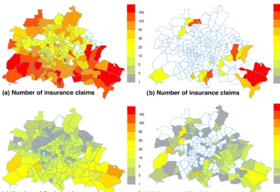
Jan-uary 2007) and the thunderstorms related to the frontal pas-sage of Gunnar (22 June 2011) can be found in Fig. 1. In general, a rather good agreement in the patterns of the num-ber of operations per zip code area and the numnum-ber of insur-ance claims is found. For Kyrill, both data sets show consid-erably higher impacts in the south of Berlin, while central and some northern parts of Berlin featured lower impacts. It can be argued that there is an influence of the size of areas that is not homogeneous (particularly large areas are found in the south, while particularly small areas in central Berlin). However, the consideration of relative numbers (normaliz-ing for the zip code area) did not alter the qualitative find-ings. For the thunderstorms related to the frontal passage of Gunnar, spatial patterns also show considerable agreement. Affected areas are considerably larger when considering fire brigade operations, while building damages are more con-centrated on individual zip code areas. This might be related to localized hailfall that led to localized occurrence of build-ing damage, while precipitation and wind gusts were more widespread, leading to water-related operations and wind-induced tree fall in larger areas. A spatial correlation analy-sis is performed, correlating the number of insurance claims and the number of operations within each zip code area. We found that using different quantities (e.g. damage ratio and normalized operation densities) does not qualitatively influ-ence the correlations. Also, it must be kept in mind that these spatial correlations are evaluated only for individual events, which may thus not be generalized. Resulting spatial corre-lations for the six events are given in Table 2.

Most prominently, significant correlations are found for tree-related operations in relation to building damages. This might affirm that tree-related operations mostly represent induced tree fall, which relates directly to wind-induced building damages. For some events (Kyrill, Lothar07 and Aram), considerable correlation is found for water-related operations while for the others there is no correlation at all. While no direct water-induced damages are included in loss data set, there might be an indirect relation. For a spe-cific event, severe precipitation might coincide with hailfall, which can induce damages. For Lothar07 and Aram there are confirmed hail observations in Berlin or surrounding ar-eas. For Kyrill a study indicates that there was thunderstorm activity during the frontal passage, which might have been re-lated to hailfall (Fink et al., 2009). The authors also note that the severe precipitation could have increased damages. This might in turn explain why for Kyrill, Lothar07 and Aram, correlations for tree-related operations and building damages are particularly high.

(7)

Addi-Figure 1.Spatial comparison of the number of insurance claims(a, b)to the number of fire brigade operations(c, d)for winter storm Kyrill in 2007(a, c)and frontal passage Gunnar in 2011(b, d).

Table 2.Spatial correlations for specific events. The correlation is calculated between the number of fire brigade operations and the number of insurance claims within individual zip code areas.

Kyrill Emma Xynthia Lothar07 Aram+ Gunnar+

All operations 0.70∗∗∗ 0.20∗∗ 0.09 0.78∗∗∗ 0.57∗∗∗ 0.46∗∗∗

Water damages 0.45∗∗∗ −0.05 −0.06 0.54∗∗∗ 0.20** 0.06

Traffic obstruction 0.09 −0.08 0.11 0.45∗∗∗ 0.16* −0.04

Tree-related 0.73∗∗∗ 0.42∗∗∗ 0.28∗∗∗ 0.79∗∗∗ 0.79∗∗∗ 0.58∗∗∗

Construction element 0.03 −0.04 −0.1 0.21** 0.19* −0.07

Others 0.06 −0.05 −0.01 −0.06 0.17∗ 0.01

Significance is indicated ifpvalue is below 0.05 (∗), below 0.01 (∗∗) and below 0.001 (∗∗∗).

tional factors might distort the relationship between insured damages and operations. These include the fact that in the case of major events both insurers and emergency services might alter their usual procedural strategies. For instance, insurers forego detailed plausibility checks for individual damage reports in the case of cumulative loss events. Also, emergency services request the public to handle non-life-threatening damage by themselves in certain situations to re-lieve workload for first responders. Both reasons might have contributed to the fact that for Kyrill an extremely high in-sured loss has been recorded (about 10 times higher com-pared to Lothar07) while the number of fire brigade opera-tions is not as exceptional (comparable to Lothar07).

4.2 Spatial correlation between potential vulnerability predictors and patterns of operation occurrences

(8)

Figure 2.Mean yearly density of fire brigade operations during 2002–2011 calculated on a 1×1 km grid (units: operations per square kilometre per year). Operation recordings are available for Berlin only (boundaries are indicated by black solid lines); i.e. zero values outside of Berlin are due to unavailability of data. Note the different colouring scale due to the fact that the absolute numbers of operations for a certain operation type vary considerably.

former airport Tempelhof. Considering individual alert key-words shows that patterns of the spatial densities of opera-tions considerably vary. While water-related operaopera-tions show a rather similar spatial pattern compared with all operations, operations related to traffic-obstructions or tree fall are dis-tributed rather differently. Both are disdis-tributed more broadly over the area of Berlin, not featuring the distinct concentra-tion in the centre. Furthermore, for operaconcentra-tions related to traf-fic obstructions a concentration of emergency operations near important junctions can be found (Fig. 2c). For tree-related operations, it seems that maxima of operation occurrence are not found in forest areas themselves but rather at their bor-ders with housing areas (e.g. compare the border areas of the Grunewald in Fig. 2d). This is not unexpected, since major impacts due to tree fall are not expected in wooden areas but rather in areas where trees are present in the direct vicinity

of man-made structures (e.g. roadside trees or trees in recre-ational areas). This implies that only in very few cases can the modelling of vulnerabilities to (meteorological) hazards be made in a univariate fashion. Instead, combinations of multiple factors will determine local vulnerability and con-sequently those that should be considered.

(9)

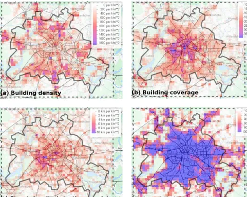
ar-Figure 3.Example set of exposure predictors calculated on a 1×1 km grid. While building density(a), building coverage(b)and street density for tertiary roads and higher(c)are based on information extracted from OpenStreetMap data, panel(d)shows the area fraction of artificial surfaces as derived from the CORINE land cover data set.

eas with concentrated large buildings. Similarly, information on the density of the road network can be derived from Open-StreetMap (Fig. 3c). Additional predictor variables from the CORINE land cover data set are assessed by calculating the fraction of a grid box that is covered by areas of a specific CORINE land use type (as one example, Fig. 3d shows the area fraction of artificial surfaces). Again, quite different in-formation can be gathered, e.g. when considering the differ-ent land use types encoded in CORINE. Finally, with respect to the aim of modelling local vulnerabilities, the characteris-tics of the local urban structure can be described on the basis of not one but instead many of these predictor variables.

For the predictor variables listed in Table 3, the spatial cor-relation to the gridded operations densities is calculated. For this, only those grid points within Berlin are considered for which data on operations are available. Furthermore, corre-lation is assessed for individual alert keywords, as well as

(10)

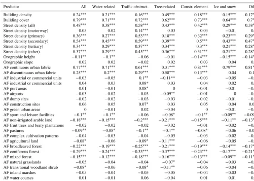
Table 3.Spatial correlation coefficients (Pearson correlation) between yearly averaged operation density with exposure predictors. Some CORINE classes are excluded in this table, if there are no areas in Berlin, and thus the area fraction (AF) is 0 everywhere. High and low correlations are highlighted in red and blue, respectively.

Predictor All Water-related Traffic obstruct. Tree-related Constr. element Ice and snow Other

Building density 0.24∗∗∗ 0.21∗∗∗ 0.16∗∗∗ 0.49∗∗∗ 0.18∗∗∗ 0.15∗∗∗ 0.17∗∗∗ Building cover 0.79∗∗∗ 0.71∗∗∗ 0.72∗∗∗ 0.62∗∗∗ 0.73∗∗∗ 0.64∗∗∗ 0.7∗∗∗ Street density (all) 0.48∗∗∗ 0.38∗∗∗ 0.58∗∗∗ 0.43∗∗∗ 0.42∗∗∗ 0.29∗∗∗ 0.38∗∗∗ Street density (motorway) 0.05 0.02 0.14∗∗∗ 0.03 0.03 −0.01 0.01 Street density (primary) 0.36∗∗∗ 0.27∗∗∗ 0.53∗∗∗ 0.18∗∗∗ 0.32∗∗∗ 0.23∗∗∗ 0.29∗∗∗ Street density (secondary) 0.54∗∗∗ 0.45∗∗∗ 0.59∗∗∗ 0.39∗∗∗ 0.5∗∗∗ 0.43∗∗∗ 0.47∗∗∗ Street density (tertiary) 0.34∗∗∗ 0.29∗∗∗ 0.37∗∗∗ 0.34∗∗∗ 0.3∗∗∗ 0.21∗∗∗ 0.28∗∗∗ Street density (other) 0.37∗∗∗ 0.29∗∗∗ 0.45∗∗∗ 0.36∗∗∗ 0.31∗∗∗ 0.21∗∗∗ 0.28∗∗∗ Orographic height −0.11∗∗ −0.1∗∗ −0.06 −0.01 −0.14∗∗∗ −0.15∗∗∗ −0.14∗∗∗ Orographic slope 0.02 0.02 −0.02 0.02 0.03 0.04 0.03 AF continuous urban fabric 0.77∗∗∗ 0.71∗∗∗ 0.61∗∗∗ 0.31∗∗∗ 0.81∗∗∗ 0.79∗∗∗ 0.81∗∗∗ AF discontinuous urban fabric 0.25∗∗∗ 0.2∗∗∗ 0.29∗∗∗ 0.58∗∗∗ 0.13∗∗∗ 0.04 0.1∗∗ AF industrial or commercial units −0.03 −0.05 0.1∗∗ −0.11** −0.03 −0.05 −0.06 AF industrial or commercial units 0.04 0.03 0.08* 0.03 0.04 0.02 0.03 AF port areas 0.01 −0.01 0.08∗ 0 −0.01 −0.01 −0.01 AF airports −0.03 −0.02 −0.03 −0.09∗∗ −0.01 0 −0.01 AF dump sites −0.02 −0.02 −0.03 −0.03 −0.02 −0.01 −0.02 AF construction sites 0.06 0.05 0.07∗ 0.03 0.05 0.04 0.08∗ AF green urban areas 0 −0.01 0.02 −0.04 0 −0.01 −0.01 AF sport and leisure facilities −0.1∗∗ −0.1∗∗ −0.06 −0.08∗ −0.1∗∗ −0.09∗∗ −0.09∗∗ AF non-irrigated arable land −0.18∗∗∗ −0.15∗∗∗ −0.2∗∗∗ −0.21∗∗∗ −0.15∗∗∗ −0.11∗∗ −0.13∗∗∗ AF fruit trees and berry plantations −0.02 −0.02 −0.02 −0.02 −0.01 −0.02 −0.02 AF pastures −0.09∗∗ −0.08∗ −0.1∗∗ −0.1∗∗ −0.08∗ −0.06 −0.07∗ AF complex cultivation patterns −0.04 −0.03 −0.04 −0.05 −0.03 −0.02 −0.03 AF agricultural land −0.08∗ −0.06 −0.09∗ −0.11∗∗∗ −0.06 −0.05 −0.06 AF broadleaved forest −0.22∗∗∗ −0.19∗∗∗ −0.25∗∗∗ −0.21∗∗∗ −0.19∗∗∗ −0.14∗∗∗ −0.17∗∗∗ AF coniferous forest −0.29∗∗∗ −0.24∗∗∗ −0.33∗∗∗ −0.37∗∗∗ −0.23∗∗∗ −0.17∗∗∗ −0.21∗∗∗ AF mixed forest −0.15∗∗∗ −0.12∗∗∗ −0.18∗∗∗ −0.16∗∗∗ −0.13∗∗∗ −0.09∗∗ −0.11∗∗∗ AF natural grasslands −0.05 −0.04 −0.04 −0.07∗ −0.04 −0.03 −0.03 AF transitional woodland shrub −0.08∗ −0.06 −0.08∗ −0.11∗∗ −0.06 −0.04 −0.05 AF inland marshes −0.05 −0.04 −0.05 −0.05 −0.04 −0.03 −0.03 AF water courses 0.01 −0.01 0.06 −0.04 0.01 0.01 0.01 AF water bodies −0.17∗∗∗ −0.14∗∗∗ −0.2∗∗∗ −0.2∗∗∗ −0.14∗∗∗ −0.09∗ −0.12∗∗∗

Significance is indicated ifpvalue is below 0.05 (∗_{), below 0.01 (}∗∗_{) and below 0.001 (}∗∗∗_).

and indicated by continuous urban fabric areas) plays a major role in determining highly vulnerable areas. Both variables can be interpreted as a proxy for the number of “objects” at harm (e.g. the number of basements or drainage systems in the case of water-related emergencies). For tree-related oper-ations, the picture is quite different, however. Operation den-sities are particularly high in areas of discontinuous urban fabric and seem to be enhanced in areas of high building den-sities (i.e. the number of houses per square kilometre). Both indicate that tree-related operations are more likely in less densely covered urban areas, where assumedly more road-side trees or trees as part of recreational areas can be found in close vicinity to building structures. Considering area frac-tion of wooded areas (particularly coniferous forests), neg-ative correlations with operations of all alert keywords are found. This can be explained by the fact that this variable is essentially inverted in areas with a high fraction covered by urban structures. Interestingly, tree-related operations are

(11)

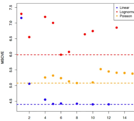
Figure 4.Results of the iterative procedure to optimize the regres-sion model. Increasing the penalty term for additional predictors leads to a model with smaller sets of predictor variables. For each of the resulting predictor sets and the corresponding multiple regres-sion, the mean cross-validation error (MSCVE) is calculated and plotted here. Blue circles represent validation results using a lin-ear regression, orange circles represent results using the lognormal model and red circles represent results using a poisson regression.

variability of weather impacts. This shall be investigated in the following by building multivariate models to statistically describe the spatial patterns of operation occurrences.

4.3 Multivariate modelling of the occurrence of fire brigade operations

The set of predictors described above is used to set up a mul-tivariate model to be able to predict the local occurrence rate of operations. As described in Sect. 3, the iterative procedure consists of the repeated application of a parameter selection algorithm while iteratively increasing the penalty for addi-tional model parameters. The optimal model is then chosen by means of the cross-validation error (to prevent overfitting and estimate the predictive ability of the resulting model). As an example, the results of this iterative procedure are shown in Fig. 4 for water-related operations. For the linear model the optimal model is identified having 12 predictor variables (which is the result of choosingk=1 as the penalty weight). Choosing a lower weight of 0 obviously results in a model taking into account all 33 possible predictors featuring severe overfitting (mean square cross-validation error (MSCVE) is about 4000 in this case). The procedure is applied to fire brigade operations associated with individual alert keywords, as well as all operations together. For the latter, the resulting optimal model includes a set of 12 predictor variables (listed in Table 4), explaining 83 % of the variance in the spatial

pat-tern of operations. In accordance to the correlation analysis, the predictor “building coverage” possesses the highest con-tribution to the explained variation (EV=59 %) while lower contributions are found for other variables (e.g. “area frac-tion continuous urban fabric” contributes 11 % and “building density” 6 %). Of course, there is not a direct correspondence when comparing the EV of individual predictor variables to the correlations as listed in Table 4, since certain predictor variables might be strongly correlated (multicollinearity; see Sect. 3.3). By adding a predictor which is correlated to pre-dictors already in the model, the increase in model perfor-mance might be small even though the correlation to the pre-dictant is high. The results described above apply to a basic linear model. Alternatively, the predictor selection method-ology can be applied while using alternative models, i.e. a log-normal and a Poisson model. Results showed that, in gen-eral, predictive abilities of the statistical models (in terms of the cross-validation error) are not increased (not shown). By means of the MSCVE, the linear models appear to perform best. However, the linear model suffers from the disadvan-tage of predicting negative values for the number of emer-gency calls in some cases, while both log-normal and Pois-son models do not. It should be noted that the different mod-els may contain a different set and even different number of predictors. The comparison of individual regression param-eters is thus difficult. However, models can be compared in terms of their predictive skill. In the following, results are shown using the linear model, performing best in terms of the predictive skill (assessed by means of the MSCVE).

In comparison with the maps shown in Fig. 2, Fig. 5 shows model predictions for the average number of operations on a 1×1 km grid cell. In the case considering all emergency op-erations (Fig. 5a) or only water related (Fig. 5b), the model nicely reproduces the concentration of operation occurrences in central parts of Berlin, while especially forest areas such as the Grunewald feature very low occurrence rates. In addi-tion, the amplitude of this variation (ranging from 0 to about 80 operations per km2 per year considering all operations) is well captured. Individual hotspots of high operation oc-currence rates, however, are only partly reproduced. This is particularly the case for a hotspot in the south-east of Berlin centre (Fig. 2a and b, corresponding to northern parts of the district Neukölln). In this area particularly, water-related op-erations are very high. It is possible that this is influenced by an extraordinarily high population density in these areas, in-formation which is only partly (and indirectly) covered by predictor variables such as building coverage. Also, other factors such as housing conditions or very localized troughs (potentially leading to water accumulation in the case of se-vere rain) might also affect the occurrence of emergency op-erations. Such information, however, was available for this study and thus cannot be taken into account.

(12)

Table 4.Resulting optimal models. First column indicates the number of predictors as well as the total explained variation (EV) of the chosen optimal model (according to the cross-validation error). The leading predictors of each model are shown indicating weather a positive (+)or negative effect (−) is found. In the last column, EV in percent is given for these leading predictors. Within the table, predictors are shown if they have an EV>1 %.

Model Predictor Estimate Std. error Significance EV (%)

All operations Building cover 12.7 6.5 ∗∗∗ 58.8

12 predictors; EV: 83 % Area fraction “continuous urban fabric” 31.6 3.0 ∗∗∗ 10.8

Building density −0.0031 0.0009 ∗∗∗ 5.9

Area fraction “industrial or commercial units” −22.8 1.9 ∗∗∗ 2.8

Street density (secondary) 2.01 0.26 ∗∗∗ 2.6

Street density (primary) 1.72 0.34 ∗∗∗ 1.2

Water-related Building cover 62.3 3.8 ∗∗∗ 47.8

7 predictors, EV: 69 % Area fraction “industrial or commercial units” −11.3 1.1 ∗∗∗ 11.3

Area fraction “continuous urban fabric” 12.2 1.8 ∗∗∗ 1.7

Area fraction “discontinuous urban fabric” −11.3 1.1 ∗∗∗ 1.5

Traffic obstruction Building cover 14.1 1.3 ∗∗∗ 53.9

8 predictors, EV: 78 % Street density (primary) 1.65 0.08 ∗∗∗ 9.3

Street density (motorway) 1.0 0.1 ∗∗∗ 1.5

Tree-related Building cover 11.4 0.6 ∗∗∗ 38.7

4 predictors, EV: 53 % Area fraction “discontinuous urban fabric” 1.4 0.1 ∗∗∗ 9.5

Construction element Building cover 23.2 1.2 ∗∗∗ 54.3

Building density −0.0005 0.0001 ∗∗ 3.2

Ice and snow Building cover 4.5 0.3 ∗∗∗ 40.4

8 predictors, EV: 72 % Area fraction “continuous urban fabric” 1.9 0.2 ∗∗∗ 24.7

Street density (all) −0.006 0.002 ∗ 1.6

Others Building cover 14.8 0.9 ∗∗∗ 48.5

Area fraction “sport and leisure facilities” −1.1 0.3 ∗∗∗ 1.1

Significance is indicated ifpvalue is below 0.05 (∗), below 0.01 (∗∗) and below 0.001 (∗∗∗).

concentrated in central parts of Berlin but are more widely distributed across Berlin. Particularly in the case of tree-related operations, model predictions show a rather homoge-neous distribution over large parts of Berlin (Fig. 5d), while local maxima in the observed operation density (Fig. 2d) are poorly captured. Considering the EV for the different mod-els, it is confirmed that for tree-related operations the predic-tive ability of the model is the worst, with an EV of 53 %. In

comparison, the model for all operations has an EV of 83 % (Table 4).

5 Conclusions and discussion

(13)

pat-Figure 5.Modelled mean yearly density of fire brigade operations (units: operations per square kilometre per year). Results are shown for the model including all operations disregarding their type(a), for water-related operations(b), for traffic obstructions(c)and for tree-related operations(d).

terns can be derived and correspondences amongst both im-pact data sets can be found. However, a complex interplay of meteorological conditions leads to a variety of weather im-pacts, making it very hard to directly compare the data sets. Instead, the availability of both data sets might be consid-ered as particularly valuable for the reconstructing the multi-faceted impacts of severe weather events.

The relation to predictor variables (i.e. the structure of settlement as well as characteristics of land use) has been addressed by means of an analysis of spatial correlations. Particularly the information on the local building coverage shows a rather high influence on the occurrence of opera-tions. Accordingly, areas classified as continuous urban fab-ric (within the CORINE land cover data set) exhibit high rates of fire brigade operations. By analysing individual alert keywords, other variables turn out as valuable predictors. For

example, in the case of traffic-related operation these include the local density of the road network. In the case of tree-related operations, the areas classified as discontinuous urban fabric correlate with high occurrence rates. One interpreta-tion is that in these areas a higher number of trees are present in the direct vicinity of man-made structures (e.g. roadside trees or trees in recreational areas).

(14)

Ex-cept for tree-related operations, the amplitude of variations can also be reproduced. However, individual hotspots with high occurrence rates are only insufficiently predicted, indi-cating that particular information influencing the local vul-nerabilities is not included in the predictor variables avail-able in this study. In the case of water-related operations, these might include housing conditions. Also, information on local tree stocks, particularly in the vicinity of vulnerable structures might be very valuable to better model tree-related operation occurrences.

Table 4 serves as an overview of the most relevant param-eters to describe the local vulnerability to severe weather, which can be the starting point for further investigations. While many details on individual predictor variables and their descriptive power with respect to specific types of oper-ations are available, a common feature is identified, namely the fact that the building coverage is by far the most dominant factor to describe the local vulnerability.

The model has been developed and tested for the Berlin area due to the availability of fire brigade operation records for Berlin. However, model predictions can be derived for the whole of Germany. Such model predictions might be par-ticularly valuable for regions with no systematic records on weather impacts. However, such extrapolation might suffer from potentially severe limitations. The occurrence of se-vere weather conditions is not homogenous over Germany, with storm frequencies being higher in northern regions and thunderstorm frequencies being higher in southern regions. Thus, the distribution of hazards causing local impacts can differ considerably, which will certainly affect the occurrence of emergency operations. Such effects are excluded in the presented modelling approach, which assume a homogenous distribution of hazards. For the investigation of Berlin this is certainly a valid assumption. The extraction of model pre-dictions for other urban areas might suffer from an offset in terms of absolute number of operations. Such model pre-dictions can, however, still be very valuable since they can provide information on spatial variation in operation occur-rences on a sub-city scale. Still, future work should include meteorological and climatological information on different hazards, which will strongly influence local vulnerability and thus predicted weather impacts.

The presented model to predict the local vulnerability to severe weather can serve as a basis for a broad range of tools or applications in emergency management. These might include tools for the long-term resource planning of lo-cal emergency management capacities. Also, handling short-term variations in the demand of local emergency manage-ment capacities might be supported by such tools when in-cluding actual weather information. In this study, we fo-cussed on data sets which are publicly available – partly open-source community data – for at least the whole of Eu-rope. This yields great potential for the design of national or even pan-European tools and applications in emergency management.

Data availability. The dataset on weather related operations of the Berlin fire department is not publicly available due to the sensitiv-ity of data. Inquiries concerning data usage should be directed to the Berlin fire brigade. The data set on insured losses is property of the Gesamtverband der Deutschen Versicherungswirtschaft e.V. (GDV) and not available to the public. Inquiries concerning data usage should be directed to GDV. Open Street Map data is freely available for download at: http://www.openstreetmap.org. Techni-cal details on the CORINE Landcover dataset can be found in Büt-tner et al. (2012) and data is available at: https://www.eea.europa.eu/ data-and-maps/data/clc-2006-vector-data-version-2. Data from the digital elevation model dgm200 (GeoBasis-DE/BKG 2016) can be retrieved from the Geodatenzentrum (http://www.geodatenzentrum. de/). The GTOPO30 dataset is available at: https://lta.cr.usgs.gov/ GTOPO30.

Competing interests. The authors declare that they have no conflict of interest.

Acknowledgements. This research was carried out in the Hans-Ertel-Centre for Weather Research (Simmer et al., 2016). This research network of Universities, Research Institutes and the Deutscher Wetterdienst is funded by the BMVI (Federal Ministry of Transport and Digital Infrastructures). We wish to thank the Gesamtverband der Deutschen Versicherungswirtschaft e.V. (GDV) for providing the loss data and for many useful discussions. We thank the Berlin fire brigade to provide the data set on weather-related operations. Finally, we thank Olga Petrucci and one anonymous reviewer for their helpful comments as well as Vassiliki Kotroni for editing our manuscript and therefore helped to improve this paper.

Edited by: Vassiliki Kotroni

Reviewed by: Olga Petrucci and one anonymous referee

References

Akaike, H.: Prediction and entropy, in: A Celebration of Statistics, edited by: Atkinson, A. C. and Fienberg, S. E., Springer, 1–24, 1985.

Aller, D. and Kozlowski, E.: Unwetter und ihre Relevanz für die Versicherungswirtschaft (Thunderstorms and their implications for the insurance industry) Promet, 34, 10–20, 2008.

Apel, H., Aronica, G. T., Kreibich, H., and Thieken, A. H.: Flood risk analyses – how detailed do we need to be?, Nat. Hazards, 49, 79–98, 2009.

Bassil, K. L., Cole, D. C., Moineddin, R., Lou, W., Craig, A. M., Schwartz, B., and Rea, E.: The relationship between temperature and ambulance response calls for heat-related illness in Toronto, Ontario, 2005, J. Epidemiol. Commun. H., 65, 829–831, 2011. Belsley, D. A., Kuh, E., and Welsch, R. E.: Regression Diagnostics:

Identifying Influential Data and Sources of Collinearity, New York, Wiley, ISBN:0-471-05856-4, 1980.

(15)

Busch, S.: Quantifying the risk of heavy rain: Its contribution to damage in urban areas, 11 th International Conference on Urban Drainage, Edinburgh, Scotland, UK, 2008.

Büttner, G., Kosztra, B., Maucha, G., Pataki, R.: Implementation and achievements of CLC2006, European Environment Agency, 2012.

CEC (Commission of the European Communities): CORINE land cover, Technical guide, Luxembourg, Office for Official Publica-tions of European Communities, 1994.

Dolney, T. J. and Sheridan, S. C.: The relationship between extreme heat and ambulance response calls for the city of Toronto, On-tario, Canada Environ. Res., 101, 94–103, 2006.

Donat, M. G., Pardowitz, T., Leckebusch, G. C., Ulbrich, U., and Burghoff, O.: High-resolution refinement of a storm loss model and estimation of return periods of loss-intensive storms over Germany, Nat. Hazards Earth Syst. Sci., 11, 2821–2833, https://doi.org/10.5194/nhess-11-2821-2011, 2011.

Fink, A. H., Brücher, T., Ermert, V., Krüger, A., and Pinto, J. G.: The European storm Kyrill in January 2007: synoptic evolution, meteorological impacts and some considerations with respect to climate change, Nat. Hazards Earth Syst. Sci., 9, 405–423, https://doi.org/10.5194/nhess-9-405-2009, 2009.

Horn, B. K. P.: Hill shading and the reflectance map, Proceedings of the IEEE 69, 14–47, 1981.

Jongman, B., Kreibich, H., Apel, H., Barredo, J. I., Bates, P. D., Feyen, L., Gericke, A., Neal, J., Aerts, J. C. J. H., and Ward, P. J.: Comparative flood damage model assessment: towards a Eu-ropean approach, Nat. Hazards Earth Syst. Sci., 12, 3733–3752, https://doi.org/10.5194/nhess-12-3733-2012, 2012.

Klawa, M. and Ulbrich, U.: A model for the estimation of storm losses and the identification of severe winter storms in Germany, Nat. Hazards Earth Syst. Sci., 3, 725–732, https://doi.org/10.5194/nhess-3-725-2003, 2003.

Kox, T., Heisterkamp, T., and Ulbrich, T.: Viel Wind um nichts? Orkan XAVER über Berlin, edited by: Gerhold, L., Jäckel, H., Schiller, J., and Steiger, S., Ergebnisse interdisziplinärer Risiko-und Sicherheitsforschung, Eine Zwischenbilanz des Forschungs-forum Öffentliche Sicherheit (Schriftenreihe Sicherheit, 17), 73– 94, 2015.

Kunz, M. and Puskeiler, M.: High-resolution assessment of the hail hazard over complex terrain from radar and insurance data Me-teorologische Zeitschrift, 19, 427–439, 2010

Pardowitz, T. and Göber, M.: Forecasting Weather Related Fire Brigade Operations on the Basis of Nowcasting Data, in: LNIS Vol. 8, RIMMA Risk Information Management, Risk Models, and Applications, CODATA Germany, Berlin, edited by: Kre-mers, H. and Susini, A., ISBN:978-3-00-056177-1, 2017.

Pinto, J. G., Neuhaus, C. P., Leckebusch, G. C., Reyers, M., and Kerschgens, M.: Estimation of wind storm impacts over West-ern Germany under future climate conditions using a statistical-dynamical downscaling approach, Tellus A, 62A, 188–201, 2010.

Rossi, P. J., Hasu, V., Halmevaara, K., Makela, A., Koistinen, J., and Pohjola, H.: Real-Time Hazard Approximation of Long-Lasting Convective Storms Using Emergency Data, J. Atmos. Ocean. Tech., 30, 538–555, 2013.

Schaffer, A., Muscatello, D., Broome, R., Corbett, S., and Smith, W.: Emergency department visits, ambulance calls, and mortal-ity associated with an exceptional heat wave in Sydney, Aus-tralia, 2011: a time-series analysis, Environ. Health, 11, 3, https://doi.org/10.1186/1476-069X-11-3, 2012.

Schuster, S. S., Blong, R. J., Leigh, R. J., and McAneney, K. J.: Characteristics of the 14 April 1999 Sydney hailstorm based on ground observations, weather radar, insurance data and emergency calls, Nat. Hazards Earth Syst. Sci., 5, 613–620, https://doi.org/10.5194/nhess-5-613-2005, 2005.

Simmer, C., Adrian, G., Jones, S., Wirth, V., Göber, M., Hoheneg-ger, C., Janjic, T., Keller, J., Ohlwein, C., Seifert, A., Trömel, S., Ulbrich, T., Wapler, K., Weissmann, M., Keller, J., Masbou, M., Meilinger, S., Riß, N., Schomburg, A., Vormann, A., and We-ingärtner, C.: HErZ – The German Hans-Ertel Centre for Weather Research, B. Amer. Met. Soc., 97, 1057–1068, 2016.

Thornes, J. E., Fisher, P. A., Rayment-Bishop, T., and Smith, C.: Ambulance call-outs and response times in Birmingham and the impact of extreme weather and climate change, Emerg. Med. J., 31, 220–228, 2014.

UNISDR United Nations Office for Disaster Risk Reduction: Sendai Framework for Disaster Risk Reduction 2015–2030, adopted at the Third United Nations World Conference on Disaster Risk Reduction in Sendai, Japan, on March 18, www. preventionweb.net/files/43291_sendaiframeworkfordrren.pdf, 2015. (last access: September 2016)

Wapler, K., Harnisch, F., Pardowitz, T., and Senf, F.: Characterisation and predictability of a strong and a weak forcing severe convective event – a multi-data approach, Meteorologische Zeitschrift, 24, 393–410, http://doi.org/10.1127/metz/2015/0625, 2015.

Wargon, M., Guidet, B., Hoang, T. D., and Hejblum, G.: A system-atic review of models for forecasting the number of emergency department visits, Emerg. Med. J., 26, 395–399, 2009.