L
L
L
e
e
e
s
s
s
c
c
c
a
a
a
h
h
h
i
i
i
e
e
e
r
r
r
s
s
s
d
d
d
u
u
u
l
l
l
a
a
a
b
b
b
o
o
o
r
r
r
a
a
a
t
t
t
o
o
o
i
i
i
r
r
r
e
e
e
L
L
L
e
e
e
i
i
i
b
b
b
n
n
n
i
i
i
z
z
z
Bayesian Robots Programming
Olivier Lebeltel
Pierre Bessière
Julien Diard
Emmanuel Mazer
Laboratoire Leibniz-IMAG, 46 av. Félix Viallet, 38000 GRENOBLE, France
-n°
01
Cahiers du Laboratoire LEIBNIZ
Bayesian Robots Programming
Olivier Lebeltel [email protected]
Pierre Bessière [email protected]
Julien Diard [email protected]
Laboratoire LEIBNIZ - CNRS
46 avenue Félix Viallet ; 38031 Grenoble ; FRANCE
Emmanuel Mazer [email protected]
Laboratoire GRAVIR - CNRS
INRIA Rhône-Alpes, ZIRST, 38030 Montbonnot
Abstract
We propose a new method to program robots based on Bayesian inference and learning. The capacities of this programming method are demonstrated through a succession of increasingly complex experiments. Starting from the learning of simple reactive behaviors, we present instances of behavior combinations, sensor fusion, hierarchical behavior com-position, situation recognition and temporal sequencing. This series of experiments comprises the steps in the incremental development of a complex robot program. The advantages and drawbacks of this approach are discussed along with these different exper-iments and summed up as a conclusion. These different robotics programs may be seen as an illustration of probabilistic programming applicable whenever one must deal with prob-lems based on uncertain or incomplete knowledge. The scope of possible applications is obviously much broader than robotics.
1. Introduction
By inference we mean simply: deductive reasoning whenever enough information is at hand to permit it; inductive or probabilistic reasoning when - as is almost invariably the case in real problems - all the necessary information is not available. Thus the topic of "Probability as Logic" is the optimal processing of uncertain and incomplete knowledge.
E.T. Jaynes1
We assume that any model of a real phenomenon is incomplete. There are always some
hid-den variables, not taken into account in the model, that influence the phenomenon. The effect of these hidden variables is that the model and the phenomenon never have the same behav-ior.
Any robot system must face this central difficulty: how to use an incomplete model of its environment to perceive, infer, decide and act efficiently? We propose an original robot pro-gramming method that specifically addresses this question.
Rational reasoning with incomplete information is quite a challenge for artificial sys-tems. The purpose of Bayesian inference and learning is precisely to tackle this problem with a well-established formal theory. Our method heavily relies on this Bayesian framework.
Lebeltel, Bessière, Diard & Mazer
We present several programming examples to illustrate this approach and define
descrip-tions as generic programming resources. We show that these resources can be used to
incre-mentally build complex programs in a systematic and uniform framework. The system is based on the simple and sound basis of Bayesian inference. It obliges the programmer to explicitly state all assumptions that have been made. Finally, it permits effective treatment of incomplete and uncertain information when building robot programs.
The paper is organized as follows. Section 2 offers a short review of the main related work, Section 3 is dedicated to definitions and notations and Section 4 presents the experi-mental platform. Sections 5 to 10 present various instances of Bayesian programs: learning simple reactive behaviors; instances of behavior combinations; sensor fusion; hierarchi-cal behavior composition; situation recognition; and temporal sequencing. Section 11 describes a combination of all these behaviors to program a robot to accomplish a night watchman task. Finally, we conclude with a synthesis summing up the principles, the theo-retical foundations and the programming method. This concluding section stresses the main advantages and drawbacks of the approach.
2. Related work
Our work is based on an implementation of the principle of the Bayesian theory of probabil-ities.
In physics, since the precursory work of Laplace (1774; 1814), numerous results have been obtained using Bayesian inference techniques (to take uncertainty into account) and the maximum entropy principle (to take incompleteness into account). The late Edward T. Jaynes proposed a rigorous and synthetic formalization of probabilistic reasoning with his "Proba-bility as Logic" theory (Jaynes, 1998). A historical review of this approach was offered by Jaynes (1979) and an epistemological analysis, by Matalon (1967). Theoretical justifications of probabilistic inference and maximum entropy are numerous. The entropy concentration theorems (Jaynes, 1982; Robert, 1990) are among the more rigorous, Cox theorem (Cox, 1961) being the most well known, although it has been partially disputed recently by Halpern (1999a; 1999b). Numerous applications and mathematical tools have been developed (Smith & Grandy, 1985; Tarentola, 1987; Bretthorst, 1988; Erickson & Smith, 1988a; Erickson & Smith, 1988b; Mohammad-Djafari & Demoment, 1992; Kapur & Kesavan, 1992).
In artificial intelligence, the importance of reasoning with uncertain knowledge has been recognized for a long time. However, the Bayesian approach clearly appeared as one of the principle trends only since the proposal of Bayesian nets (Pearl, 1988) and graphical models (Lauritzen & Spiegehalter, 1988; Lauritzen, 1996; Jordan, 1998; Frey, 1998). Very important technical progress has been achieved recently (See for instance the JAIR2 articles on that subject: Saul et al., 1996; Zhang & Poole, 1996; Delcher et al., 1996; Darwiche & Provan, 1997; Ruiz et al., 1998; Jaakola & Jordan, 1999; Jordan et al., 1999).
Recent robot programming architectures (Alami et al., 1998; Borrelly et al., 1998; Schneider et al., 1998; Dekhil & Henderson, 1998; Mazer et al., 1998) are in general not concerned with the problem of uncertainty. In robotics, the uncertainty topic is either related to calibration (Bernhardt & Albright, 1993) or to planning problems (Brafman et al., 1997). In the latter case, some authors have considered modeling the uncertainty of the robot motions when planning assembly operations (Lozano-Perez et al., 1984; Donald, 1988) or modeling the uncertainty related to the position of the robot in a scene (Kapur & Kesavan,
Bayesian Robot Programming
1992). Bayesian techniques are used in POMDP3 to plan complex paths in partially known
environments (Kaelbling, Littman & Cassandra, 1996). HMM4 are also used to plan complex tasks and recognize situations in complex environments (Aycard, 1998, Thrun, 1998). How-ever, to the best of our knowledge, the design of a robot programming system and architec-ture solely based on Bayesian inference has never been investigated before.
Finally, a presentation of the epistemological foundations of the approach described in this paper may be found in two articles by Bessière et al. (1998a; 1998b) and all the technical details in the PhD dissertation of Olivier Lebeltel (1999).
3. Basic concepts
In this section, we introduce the concepts, postulates, definitions, notations and rules that are necessary to define a Bayesian robot program.
3.1 Definition and notation
Proposition
The first concept we will use is the usual notion of logical proposition. Propositions will be denoted by lowercase names. Propositions may be composed to obtain new proposition using
the usual logical operators: denoting the conjunction of propositions and ,
their disjunction and the negation of proposition .
Variable
The notion of discrete variable is the second concept we require. Variables will be denoted by names starting with one uppercase letter.
By definition, a discrete variable is a set of logical propositions such that these
propositions are mutually exclusive (for all with , is false) and exhaustive (at
least one of the propositions is true). stands for «variable takes its value». denotes the cardinal of the set (the number of propositions ).
The conjunction of two variables and , denoted , is defined as the set of
propositions . is a set of mutually exclusive and exhaustive logical
propositions. As such, it is a new variable5. Of course, the conjunction of variables is also a variable and, as such, it may be renamed at any time and considered as a unique variable in the sequel.
Probability
To be able to deal with uncertainty, we will attach probabilities to propositions.
We consider that, to assign a probability to a proposition , it is necessary to have at
least some preliminary knowledge, summed up by a proposition . Consequently, the
proba-bility of a proposition is always conditioned, at least, by . For each different ,
is an application assigning to each proposition a unique real value in the interval
.
Of course, we will be interested in reasoning on the probabilities of the conjunctions,
3. Partially Observable Markoff Decision Process 4. Hidden Markov Models
5. By contrast, the disjunction of two variables, defined as the set of propositions , is not a variable. These propositions are not mutually exclusive.
a∧b a b a∨b
a
¬ a
X xi
i j, i≠ j xi∧yj
xi xi X ith X
X xi
X Y X⊗Y
X × Y xi∧yj X⊗Y
n
xi∨yj a
π
a π π P(.|π)
a P(a|π)
0 1,
Lebeltel, Bessière, Diard & Mazer
disjunctions and negations of propositions, denoted, respectively, by ,
and .
We will also be interested in the probability of proposition conditioned by both the
preliminary knowledge and some other proposition . This will be denoted .
For simplicity and clarity, we will also use probabilistic formula with variables appearing instead of propositions. By convention, each time a variable appears in a probabilistic
for-mula , it should be understood as . For instance, given three variables ,
and , stands for:
[E3.1]
3.2 Inference postulates and rules
This section presents the inference postulates and rules necessary to carry out probabilistic reasoning.
Conjunction and normalization postulates for propositions
Probabilistic reasoning needs only two basic rules:
1 - The conjunction rule, which gives the probability of a conjunction of proposi-tions.
[E3.2]
2 - The normalization rule, which states that the sum of the probabilities of and is one.
[E3.3]
For the purpose of this paper, we take these two rules as postulates6.
As in logic, where the resolution principle (Robinson, 1965; Robinson, 1979) is suffi-cient to solve any inference problem, in discrete probabilities, these two rules ([E3.2], [E3.3]) are sufficient for any computation. In particular, we may derive all the other neces-sary inference rules from those two, especially the rules concerning variables.
Disjunction rule for propositions
For instance, the rule concerning the disjunction of propositions:
[E3.4]
may be derived as follows:
6. See some references on justifications of these two rules in § 2.
a∧b|π
( )
P P(a∨b|π) a
¬ |π
( )
P
a
π b P(a|b∧π)
X
Φ( )X ∀xi∈X,Φ( )xi X Y
Z P(X⊗Y|Z⊗π) = P(X|π)
xi
∀ ∈X,∀yj∈Y,∀zk∈Z P(xi∧yj|zk∧π) = P(xi|π)
a∧b|π
( )
P = P(a|π)×P(b|a∧π) b|π
( )
P ×P(a|b∧π) =
a ¬a
a|π
( )
P +P(¬a|π) = 1
a∨b|π
( )
Bayesian Robot Programming
[E3.5]
Conjunction rule for variables
[E3.6]
According to our notation convention for probabilistic formula including variables, this may be restated as:
[E3.7]
which may be directly deduced from equation [E3.2].
Normalization rule for variables
[E3.8]
The normalization rule may obviously be derived as follows:
[E3.9]
where the first equality derives from equation [E3.3], the second from the exhaustiveness of propositions and the third from both the application of equation [E3.4] and the mutual exclusivity of propositions .
Marginalization rule for variables
[E3.10]
The marginalization rule is derived by the successive application of the product rule (equation [E3.6]) and the normalization rule (equation [E3.8]):
a∨b|π
( )
P = 1–P(¬a∧¬b|π)
1–P(¬a|π)×P(¬b|¬a∧π) =
1–P(¬a|π)×(1–P(b|¬a∧π)) =
a|π
( )
P +P(¬a∧b|π) =
a|π
( )
P +P(b|π)×P(¬a|b∧π) =
a|π
( )
P +P(b|π)×(1–P(a|b∧π)) =
a|π
( )
P +P(b|π)–P(a∧b|π) =
X⊗Y|π
( )
P = P(X|π)×P(Y|X⊗π) Y|π
( )
P ×P(X|Y⊗π)
=
xi
∀ ∈X,∀yj∈Y xi∧yj|π
( )
P = P(xi|π)×P(yj|xi∧π)
yj|π
( )
P ×P(xi|yj∧π) =
X|π
( )
P X
∑
= 11 = P(x1|π)+P(¬x1|π)
x1|π
( )
P +P(x2∨...∨x X |π) =
x1|π
( )
P +P(x2|π)+...+P(x X |π) =
xi|π
( )
P xi
∑
∈X=
xi
xi
X⊗Y|π
( )
P X
[E3.11]
3.3 Bayesian Programs
We have defined a Bayesian program as a means of specifying a family of probability distributions. Our goal is to show that by using such a specification one can effectively con-trol a robot to perform complex tasks.
The constituent elements of a Bayesian program are presented in Figure 1:
• A program is constructed from a description and a question.
• A description is constructed from preliminary knowledge and a data set.
• Preliminary knowledge is constructed from a set of pertinent variables, a decompo-sition and a set of forms.
• Forms are either parametric forms or programs.
Description
The purpose of a description is to specify an effective method to compute a joint distribution
on a set of variables given a set of experimental data and preliminary
knowl-edge . This joint distribution is denoted as: .
Preliminary Knowledge
To specify preliminary knowledge the programmer must undertake the following:
1 Define the set of relevant variables on which the joint distribution is
defined.
2 Decompose the joint distribution:
Given a partition of into subsets we define variables each
corresponding to one of these subsets.
Each variable is obtained as the conjunction of the variables belonging to
the subset . The conjunction rules [E3.6] leads to:
Figure 1: Structure of a bayesian program X⊗Y|π
( )
P X
∑
P(Y|π)×P(X|Y⊗π)X
∑
=
Y|π
( )
P P(X|Y⊗π)
X
∑
×
=
Y|π
( )
P
=
Program Description
Preliminary Knowledge ( )π
Pertinent Variables
Decomposition
Forms Parametrical Forms
Programs
Data ( )δ
Question
X1,X2, ,… Xn
{ } δ
π P(X1⊗X2⊗…⊗Xn|δ π⊗ )
X1,X2, ,… Xn
{ }
X1,X2, ,… Xn
{ } k k L1, ,… Lk
Li {Xi1,Xi2,…}
[E3.12]
Conditional independence hypotheses then allow further simplifications. A conditional
independence hypothesis for variable is defined by picking some variables
among the variables appearing in conjunction , calling the
con-junction of these chosen variables and setting:
[E3.13]
We then obtain:
[E3.14]
Such a simplification of the joint distribution as a product of simpler distributions is called a decomposition.
3 Define the forms:
Each distribution appearing in the product is then associated with
either a parametric form (i.e., a function ) or another Bayesian program. In
gen-eral, is a vector of parameters that may depend on or or both. Learning takes place when some of these parameters are computed using the data set
Question
Given a description (i.e., ), a question is obtained by
partition-ing into three sets : the searched variables, the known variables and the
unknown variables.
We define the variables , and as the conjunction of the variables
belonging to these sets. We define a question as the distribution:
. [E3.15]
3.4 Running Bayesian programs
Running a Bayesian program supposes two basic capabilities: Bayesian inference and deci-sion-making.
Bayesian inference
Given the joint distribution , it is always possible to compute
any possible question, using the following general inference: X1⊗X2⊗…⊗Xn|δ π⊗
( )
P
L1|δ π⊗
( )
P ×P(L2|L1⊗ ⊗δ π)×…×P(Lk|Lk–1⊗…⊗L2⊗L1⊗ ⊗δ π) =
Li Xj
Li–1⊗…⊗L2⊗L1 Ri
Li|Li–1⊗…⊗L2⊗L1⊗ ⊗δ π
( )
P = P(Li|Ri⊗ ⊗δ π)
X1⊗X2⊗…⊗Xn|δ π⊗
( )
P
L1|δ π⊗
( )
P ×P(L2|R2⊗ ⊗δ π)×P(L3|R3⊗ ⊗δ π)×…×P(Lk|Rk⊗ ⊗δ π) =
Li|Ri⊗ ⊗δ π
( )
P
fµ( )Li
µ Ri δ
δ
X1⊗X2⊗…⊗Xn|δ π⊗
( )
P
X1,X2,... X, n
{ }
Search Known Unknown
Searched|Known⊗ ⊗δ π
( )
P
X1⊗X2⊗…⊗Xn|δ π⊗
( )
[E3.16]
where the first equality results from the marginalization rule (equation [E3.10]), the sec-ond results from the product rule (equation [E3.6]) and the third correspsec-onds to a secsec-ond application of the marginalization rule. The denominator appears to be a normalization term. Consequently, by convention, we will replace it by .
It is well known that general Bayesian inference is a very difficult problem, which may be practically intractable. Exact inference has been proved to be NP-hard (Cooper, 1990) and the general problem of approximate inference too (Dagum & Luby, 1993). Numerous heuris-tics and restrictions to the generality of the possible inferences have been proposed to achieve admissible computation time (see the papers already cited in Section 2 about techni-cal progress in this area).
An inference engine and the associated programming API7 as been developed and used
for the experiments presented in this paper. The same API has also been used for other appli-cations such as CAD modeling (see Mekhnacha, 1999).
Our engine proceeds in two phases: a symbolic simplification phase which reduces the complexity of the considered sums, and a numeric phase that computes an approximation of the distributions.
Our symbolic simplification phase drastically reduces the number of sums necessary to compute a given distribution. However the decomposition part of the preliminary knowledge, which expresses the conditional dependencies of variables, still plays a crucial role in keep-ing the computation tractable. The importance of the decomposition has already been stressed by many authors (e.g., Zhang & Poole, 1996) and explains the good performances of our engine (10 inferences per second8).
Decision-making
For a given distribution, different decision policies are possible: for example, searching the best (highest probability) values or drawing at random according to the distribution. For our purposes, we will always use this second policy and refer this query as:
.
Control loop of the robot
To control our robot using a Bayesian program, a decision is made every tenth of a sec-ond. A typical question is to select the values of the motor variables knowing the values of
7. Application Programming Interface
8. Order of magitude on a standard desk top computer for the inferences required by the experiments described in the sequel.
Searched|Known⊗ ⊗δ π
( )
P P(Searched⊗Unknown|Known⊗ ⊗δ π)
Unknown
∑
=
Searched⊗Unknown⊗Known|δ π⊗
( )
P Unknown
∑
Known|δ π⊗
( )
P
---=
Searched⊗Unknown⊗Known|δ π⊗
( )
P Unknown
∑
Searched⊗Unknown⊗Known|δ π⊗
( )
P Searched Unknown
∑
---=
1
Σ
--- P(Searched⊗Unknown⊗Known|δ π⊗ )
Unknown
∑
×
=
Σ
the sensory variables. Consequently, the basic loop to operate the robot is to loop on the fol-lowing instructions every tenth of a second:
1 - Read the values of the sensors
2 -
3 - Send the returned values to the motors
4. Experimental platform
4.1 Khepera robot
Khepera is a two-wheeled mobile robot, 57 millimeters in diameter and 29 millimeters in height, with a total weight of 80g (See Figure 2). It was designed at EPFL9 and is commer-cialized by K-Team10.
The robot is equipped with eight light sensors (six in front and two behind), taking
val-ues between 0 and 511 in inverse relation to light intensity, stored in variables (see
Figure 3). These eight sensors can also be used as infrared proximeters, taking values between 0 and 1023 in inverse relation to the distance from the obstacle, stored in variables
(see Figure 3).
The robot is controlled by the rotation speeds of its left and right wheels, stored in vari-ables Mg and Md, respectively.
From these 18 basic sensory and motor variables, we derived three new sensory variables
( , and ) and one new motor one ( ). They are described below.
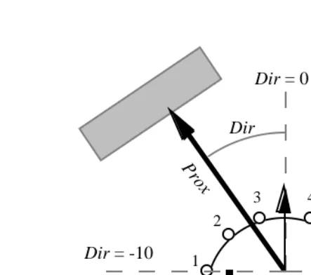
• is a variable that approximately corresponds to the bearing of the closest obsta-cle (See Figure 3). It takes values between -10 (obstaobsta-cle to the left of the robot) and +10 (obstacle to the right of the robot), and is defined as follows:
9. Ecole Polytechnique Fédérale de Lausane (Switzerland)
Figure 2: The Khepera mobile robot (from the top and from the left)
10. http://www.K-team.com/
Draw(P(Motors|Sensors⊗ ⊗δ π))
L1, ,… L8
Px1, ,… Px8
Dir Prox Theta1 Vrot
[E4.1]
• is a variable that approximately corresponds to the proximity of the closest
obstacle (See Figure 3). It takes values between zero (obstacle very far from the robot) and 15 (obstacle very close to the robot), and is defined as follows:
[E4.2]
• is a variable that approximately corresponds to the bearing of the greatest
source of illumination. It takes on 36 values from -170° to 180°.
• The robot is piloted solely by its rotation speed (the translation speed is fixed). It
receives motor commands from the variable, calculated from the difference
between the rotation speeds of the left and right wheels. takes on values
between -10 (fastest to the left) and +10 (fastest to the right).
Khepera accepts turrets on its top to augment either its sensory or motor capacities. For the final experiment (the nightwatchman task), a linear camera of 64 pixels and a micro tur-bine were added on top of the robot.
4.2 Environment
For all experiments described in the current paper, the Khepera is placed in a 1 m by 1 m environment. This environment has walls around its contour, textured to be easily seen by the robot. Inside this square, we place walls made of Lego© bricks that can be moved easily to set any configuration we need quickly. We usually build a recess made of high Lego© walls in a corner, and place a small light over this recess, to create a «base» for the robot.
Figure 3: The sensory-motor variables of the Khepera robot.
Vrot
- +
1 2
3 4
6 5
7 8
Dir
Prox
Dir = +10 Dir = 0
Dir = -10
Dir Floor 90 Px6( –Px1)+45 Px5( –Px2)+5 Px4( –Px3)
9 1( +Px1+Px2+Px3+Px4+Px5+Px6)
---
=
Prox
Prox Floor Max Px1 Px2 Px3 Px4 Px5 Px6( , , , , , )
64
---
=
Theta1
Vrot
5. Reactive behavior
5.1 Goal and experimental protocol
The goal of the first experiment was to teach the robot how to push objects.
First, in a learning phase, we drove the robot with a joystick to push objects. During that phase, the robot collected, every tenth of a second, both the values of its sensory variables and the values of its motor variables (determined by the joystick position). This data set was then used to identify the free parameters of the parametric forms.
Then, in a restitution phase, the robot has to reproduce the behavior it had just learned. Every tenth of a second it decided the values of its motor variables, knowing the values of its sensory variables and the internal representation of the task.
5.2 Specification
Having defined our goal, we describe the three steps necessary to define the preliminary knowledge.
1 - Chose the pertinent variables
2 - Decompose the joint distribution
3 - Define the Parametric forms
Variables
First, the programmer specifies which variables are pertinent for the task.
To push objects it is necessary to have an idea of the position of the objects relative to the robot. The front proximeters provide this information. However, we chose to sum up the
information of these six proximeters by the two variables and .
We also chose to set the translation speed to a constant and to operate the robot by its
rotation speed .
These three variables are all we need to push obstacles. Their definitions are summed up as follows:
[S5.1]
Decomposition
In the second specification step, we give a decomposition of the joint probability as a product of simpler terms. This distribution is
condi-tioned by both , the preliminary knowledge we are defining, and a data set that
will be provided during the learning phase.
[S5.2]
The first equality results from the application of the product rule (equation [E3.6]). The
Dir Prox
Vrot
Dir∈{–10, ,… 10}, Dir =21
Prox∈{0, ,… 15}, Prox =16 Vrot∈{–10, ,… 10}, Vrot =21
Dir⊗Prox⊗Vrot|∆⊗π-obstacle
( )
P
π-obstacle ∆
Dir⊗Prox⊗Vrot|∆⊗π-obstacle
( )
P
Dir|∆⊗π-obstacle
( )
P ×P(Prox|Dir⊗ ⊗∆ π-obstacle)×P(Vrot|Prox⊗Dir⊗ ⊗∆ π-obstacle) =
Dir|∆⊗π-obstacle
( )
second results from the simplification ,
which means that we consider that and are independent. The distances to the
objects and their bearings are not contingent.
Parametric forms
To be able to compute the joint distribution, we finally need to assign parametric forms to each of the terms appearing in the decomposition:
[S5.3]
We have no a priori information about the direction and the distance of the obstacles.
Hence, and are uniform distributions; all
direc-tions and proximities have the same probability.
For each sensory situation, we believe that there is one and only one rotation speed that
should be preferred. The distribution is unimodal. However,
depending of the situation, the decision to be made for may be more or less certain. This
is resumed by assigning a Gaussian parametrical form to .
5.3 Identification
We drive the robot with a joystick (see Movie 111), and collect a set of data . Let us call the
particular set of data corresponding to this experiment . A datum collected at time is
a triplet .
The free parameters of the parametric forms (means and standard deviations for all the Gaussians) can then be identified.
Finally, it is possible to compute the joint distribution:
[E5.1]
According to equation [E3.16], the robot can answer any question concerning this joint distribution.
We call the distribution a description of the task. A
description is the result of identifying the free parameters of a preliminary knowledge using some given data. Hence, a description is completely defined by a couple preliminary knowl-edge + data. That is why a conjunction always appears to the right of a description.
5.4 Utilization
To render the pushing obstacle behavior just learned, the Bayesian controller is called every tenth of a second :
1 - The sensors are read and the values of and are computed
2 - The Bayesian program is run with the query:
11. http://www-leibniz.imag.fr/LAPLACE/Cours/Semaine-Science/Trans7/T7.mov (QuickTime, 4.4 Mo) Prox|Dir⊗ ⊗∆ π-obstacle
( )
P = P(Prox|∆⊗π-obstacle)
Prox Dir
Dir|∆⊗π-obstacle
( )
P ≡Uniform
Prox|∆⊗π-obstacle
( )
P ≡Uniform
Vrot|Prox⊗Dir⊗ ⊗∆ π-obstacle
( )
P ≡G(µ(Prox Dir, ) σ, (Prox Dir, ))
Dir|∆⊗π-obstacle
( )
P P(Prox|∆⊗π-obstacle)
Vrot|Prox⊗Dir⊗ ⊗∆ π-obstacle
( )
P
Vrot
Vrot|Prox⊗Dir⊗ ⊗∆ π-obstacle
( )
P
∆
δ-push t
vrott,dirt,proxt
( )
Dir × Prox
Dir⊗Prox⊗Vrot|δ-push⊗π-obstacle
( )
P
Dir|π-obstacle
( )
P ×P(Prox|π-obstacle)×P(Vrot|Prox⊗Dir⊗δ-push⊗π-obstacle) =
Dir⊗Prox⊗Vrot|δ-push⊗π-obstacle
( )
P
δ π⊗
[E5.2]
3 - The drawn is sent to the motors
5.5 Results, lessons and comments
Results
As shown in Movie 111, the Khepera learns how to push obstacles in 20 to 30 seconds. It
learns the particular dependency, corresponding to this specific behavior, between the
sen-sory variables and and the motor variable .
This dependency is largely independent of the particular characteristics of the objects (weight, color, balance, nature, etc.). Therefore, as shown in Movie 212, the robot is also able to push different objects. This, of course, is only true within certain limits. For instance, the robot will not be able to push the object if it is too heavy.
Method
In this experiment we apply a precise three-step method to program the robot.
1 - Specification: define the preliminary knowledge
1.1 - Choose the pertinent variables
1.2 - Decompose the joint distribution
1.3 - Define the Parametric forms
2 - Identificationn:identify the free parameters of the preliminary knowledge
3 - Utilization: ask a question to the joint distribution
In the sequel, we will use the very same method for all the other experiments.
Variations
Numerous different behaviors may be obtained by changing some of the different compo-nents of a Bayesian program in the following ways.
• It is possible to change the question, keeping the description unchanged. For instance, if the information is no longer available because of some failure, the robot may still try to push the obstacles knowing only their direction. The query is then:
[E5.3]
• It is possible to change the data, keeping the preliminary knowledge unchanged.
For instance, with the same preliminary knowledge , we taught the robot
to avoid objects or to follow their contour (see Figure 4 and Movie 313). Two new descriptions14 were obtained by changing only the driving of the robot during the
12. http://www-leibniz.imag.fr/LAPLACE/Cours/Semaine-Science/Trans8/T8.mov (QuickTime, 1Mo) 13. http://www-leibniz.imag.fr/LAPLACE/Cours/Semaine-Science/Trans9/T9.mov (QuickTime, 3.6Mo)
14. and
Draw(P(Vrot|proxt⊗dirt⊗δ-push⊗π-obstacle))
vrott
Dir Prox Vrot
Prox
Draw(P(Vrot|dirt⊗δ-push⊗π-obstacle))
π-obstacle
Dir⊗Prox⊗Vrot|δ-avoid⊗π-obstacle
( )
learning phase. As a result, two new programs were obtained leading to the expected behaviors : «obstacle avoidance» and «contour following».
• Finally, it is possible to change the preliminary knowledge, which leads to com-pletely different behaviors. Numerous examples will be presented in the sequel of this paper. For instance, we taught the robot another reactive behavior called photo-taxy. Its goal is then to move toward a light source. This new preliminary
knowl-edge uses the variables and . roughly corresponds to
the direction of the light.
6. Behavior combination
6.1 Goal and experimental protocol
In this experiment we want the robot to go back to its base where it can recharge.
This will be obtained with no further teaching. As the robot's base is lit, the light gradient usually gives good hints on its direction. Consequently, we will obtain the homing behavior by combining together the obstacle avoidance behavior and the phototaxy behavior. By pro-gramming this behavior we will illustrate one possible way to combine Bayesian programs that make use of «command variable».
6.2 Specification
Variables
We need , , and , the four variables already used in the two composed
behaviors. We also need a new variable which acts as a command to switch from avoid-ance to phototaxy.
Figure 4: Contour following (superposed images)
π-phototaxy1 Vrot Theta1 Theta1
Dir Prox Theta1 Vrot
[S6.1]
Decomposition
We believe that the sensory variables , and are independent from one another.
Far from any objects, we want the robot to go toward the light. Very close to obstacles, we
want the robot to avoid them. Hence, we consider that should only depend on .
Finally, we believe that must depend on the other four variables. These programmer
choices lead to the following decomposition:
[S6.2]
Parametric forms
We have no a priori information about either the direction and distance of objects or the direction of the light source. Consequently, we state:
[S6.3]
is a command variable to switch from avoidance to phototaxy. This means that when the robot should behave as it learned to do in the description
and when the robot should behave
according to the description . Therefore, we state:
[S6.4]
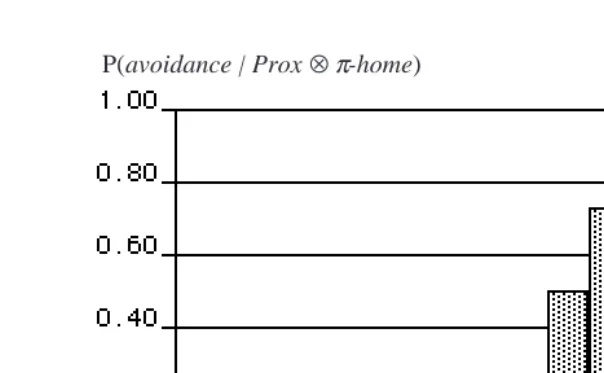
We want a smooth transition from phototaxy to avoidance as we move closer and closer to objects. Hence we finally state:
[S6.5]
The discrete approximation of the Sigmoid function we use above, which will not be defined in the current paper, is shown in Figure 5.
The preliminary knowledge is defined by specifications [S6.1], [S6.2], [S6.3],
[S6.4] and [S6.5].
6.3 Identification
There are no free parameters in preliminary knowledge . No learning is required.
Dir∈{–10, ,… 10}, Dir =21 Prox∈{0, ,… 15}, Prox =16 Theta1∈{–170, ,… 180}, Theta1 =36
Vrot∈{–10, ,… 10}, Vrot =21 H∈{avoidance phototaxy, }, H =2
Dir Prox Theta1
H Prox
Vrot
Dir⊗Prox⊗Theta1⊗ ⊗H Vrot|∆⊗π-home
( )
P
Dir|π-home
( )
P ×P(Prox|π-home)×P(Theta1|π-home)×P(H|Prox⊗π-home) =
.×P(Vrot|Dir⊗Prox⊗Theta1⊗ ⊗H π-home)
Dir|π-home
( )
P ≡Uniform
Prox|π-home
( )
P ≡Uniform
Theta1|π-home
( )
P ≡Uniform
H
H = avoidance
Dir⊗Prox⊗Vrot|δ-avoid⊗π-obstacle
( )
P H = phototaxy
Theta1⊗Vrot|δ-phototaxy⊗π-phototaxy1
( )
P
Vrot|Dir⊗Prox⊗Theta1⊗avoidance⊗π-home
( )
P ≡P(Vrot|Dir⊗Prox⊗δ-avoid⊗π-obstacle)
Vrot|Dir⊗Prox⊗Theta1⊗phototaxy⊗π-home
( )
P ≡P(Vrot|Theta1⊗δ-phototaxy⊗π-phototaxy1)
avoidance|Prox⊗π-home
( )
P ≡Sigmoidα β, (Prox) (α=9) β,( =0 25, )
phototaxy|Prox⊗π-home
( )
P = 1–P(avoidance|Prox⊗π-home)
π-home
6.4 Utilization
While Khepera returns to its base, we do not know in advance when it should avoid obstacles or when it should go toward the light. Consequently, to render the homing behavior we will use the following question where is unknown:
[E6.1]
Equation [E6.1] shows that the robot does a weighted combination between avoidance
and phototaxy. Far from any objects ( ) it does pure
phototaxy. Very close to objects ( ) it does pure
avoidance. In between, it mixes the two.
6.5 Results, lessons and comments
Results
Figure 6 and Movie 415 show efficient homing behavior obtained this way.
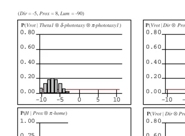
Figures 7 and 8 present the probability distributions obtained when the robot must avoid an obstacle on the left with a light source also on the left. As the object is on the left, the robot needs to turn right to avoid it. This is what happens when the robot is close to the objects (see Figure 7). However, when the robot is further from the object, the presence of the light source on the left influences the way the robot avoids obstacles. In that case, the robot may turn left despite the presence of the obstacle (see Figure 8).
Figure 5:
15. http://www-leibniz.imag.fr/LAPLACE/Cours/Semaine-Science/Trans10/T10.mov (QuickTime, 4.3Mo)
Prox
P(avoidance | Prox ⊗π-home)
avoidance|Prox⊗π-home
( )
P
H
Vrot|Dir⊗Prox⊗Theta1⊗π-home
( )
P
Vrot⊗H|Dir⊗Prox⊗Theta1⊗π-home
( )
P H
∑
=
1
Σ
--- [P(avoidance|Prox⊗π-home)×P(Vrot|Dir⊗Prox⊗δ-avoid⊗π-obstacle)]
.+[P(phototaxy|Prox⊗π-home)×P(Vrot|Theta1⊗δ-phototaxy⊗π-phototaxy1)] ×
=
Figure 6: Homing behavior (The arrow points out the light source) (superposed images).
Figure 7: Homing behavior (Khepera close to an object on its left). The top left distribution shows the knowledge on given by the phototaxy description; the top right is given by the avoidance description; the bottom left shows the knowledge
of the «command variable» ; finally the bottom right shows the resulting
combination on .
(Dir = -5, Prox = 10, Lum = -90)
0.00 0.20 0.40 0.60 0.80
-10 -5 0 5 10
0.00 0.20 0.40 0.60 0.80
-10 -5 0 5 10
0.00 0.25 0.50 0.75 1.00
0.00 0.20 0.40 0.60 0.80
-10 -5 0 5 10
phototaxyavoidance
P(Vrot | Theta1 ⊗δ-phototaxy ⊗π-phototaxy1 ) P(Vrot | Dir ⊗ Prox ⊗δ-avoid ⊗π-obstacle)
P(H | Prox ⊗π-home) P(Vrot | Dir ⊗ Prox ⊗ Theta1 ⊗π-home)
Vrot Vrot
H
Descriptions combination method
In this experiment we present a simple instance of a general method to combine descriptions to obtain a new mixed behavior. This method uses a command variable to switch from one of the composing behaviors to another. A probability distribution on knowing some sen-sory variables should then be specified or learned16. The new description is finally used by asking questions where is unknown. The resulting sum on the different cases of does the mixing.
This shows that Bayesian robot programming allows easy, clear and rigorous specifica-tions of such combinaspecifica-tions. This seems to be an important benefit compared to some other methods that have great difficulties in mixing behaviors with one another, such as Brooks’ subsumption architecture (Brooks, 1986; Maes, 1989) or neural networks. Description com-bination appears to naturally implement a mechanism similar to HEM17 (Jordan & Jacobs, 1994).
7. Sensor fusion
7.1 Goal and experimental protocol
The goal of this experiment is to fuse the data originating from the eight light sensors to Figure 8: Homing behavior (Khepera further from the object on its left).
This figure is structured as Figure 7.
16. see (Diard & Lebeltel, 1999) 17. Hierachical Mixture of Expert
(Dir = -5, Prox = 8, Lum = -90)
phototaxyavoidance
P(Vrot | Theta1 ⊗δ-phototaxy ⊗π-phototaxy1 ) P(Vrot | Dir ⊗ Prox ⊗δ-avoid ⊗π-obstacle)
P(H | Prox ⊗π-home) P(Vrot | Dir ⊗ Prox ⊗ Theta1 ⊗π-home) 0.00
0.20 0.40 0.60 0.80
-10 -5 0 5 10
0.00 0.20 0.40 0.60 0.80
-10 -5 0 5 10
0.00 0.25 0.50 0.75 1.00
0.00 0.20 0.40 0.60 0.80
-10 -5 0 5 10
H H
determine the position of a light source.
This will be obtained in two steps. In the first one, we specify one description for each sensor individually. In the second one, we mix these eight descriptions to form a global one.
7.2 Sensor model
Specification
Variables
To build a model of the light sensor , we only require two variables: the reading of the
sensor, and , the bearing of the light source.
[S7.1]
Decomposition
The decomposition simply specifies that the reading of a sensor obviously depends on the position of the light source
[S7.2]
Parametric forms
As we have no a priori information on the position of the source, we state:
[S7.3]
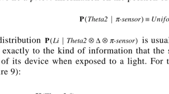
The distribution is usually very easy to specify because it
cor-responds exactly to the kind of information that the sensor supplier provides: the expected readings of its device when exposed to a light. For the Khepera’s light sensors, we obtain (see Figure 9):
Figure 9:
i Li
ith Theta2
Li∈{0, ,… 511}, Li =512 Theta2∈{–170, ,… 180}, Theta2 =36
Theta2⊗Li|∆⊗π-sensor
( )
P
Theta2|π-sensor
( )
P ×P(Li|Theta2⊗ ⊗∆ π-sensor)
=
Theta2|π-sensor
( )
P ≡Uniform
Li|Theta2⊗ ⊗∆ π-sensor
( )
P
K(Theta2,0)
Theta2 (°)
[S7.4]
In specification [S7.4], stands for the position of the sensor with respect to the robot, and will be used later to «rotate» this model for different sensors.
Specifications [S7.1], [S7.2], [S7.3] and [S7.4] are the preliminary knowledge
corre-sponding to this sensor model. This preliminary knowledge is named .
Identification
No identification is required as there are no free parameters in .
However, it may be easy and interesting to calibrate specifically each of the eight light sensors. This could be achieved, for instance, by identifying parameters and indepen-dently for each sensor, by observing the response of the particular sensor to a light source.
7.3 Fusion
Specification
Variables
The interesting variables are the eight variables and :
[S7.5]
Decomposition
The decomposition of the joint distribution is chosen to be:
[S7.6]
The first equality results from the product rule [E3.6]. The second from simplifications of the kind:
[E7.1]
These simplifications may seem peculiar as obviously the readings of the different light sensors are not independent. The exact meaning of these equations is that we consider (the position of the light source) to be the main reason for the contingency of the readings.
Consequently, we state that, knowing , the readings are independent. is the
cause of the readings and knowing the cause, the consequences are independent. This is, indeed, a very strong hypothesis. The snesors may be correlated for numerous other reasons.
Li|Theta2⊗π-sensor
( )
P ≡GK Theta2( ,θi) σ, ( )Li
K Theta2( ,θi) 1 1
1+e–4β(Theta2–θi –α) ---–
= (α=45) β,( =0 03, )
θi
π-sensor
π-sensor
α β
Li Theta2
L1∈{0, ,… 511}, L1 =512
…
L8∈{0, ,… 511}, L8 =512 Theta2∈{–170, ,… 180}, Theta2 =36
Theta2⊗L1⊗L2⊗L3⊗L4⊗L5⊗L6⊗L7⊗L8|∆⊗π-fusion
( )
P
Theta2|∆⊗π-fusion
( )
P ×P(L1|Theta2⊗ ⊗∆ π-fusion)×P(L2|L1⊗Theta2⊗ ⊗∆ π-fusion) =
…×P(L8|L7⊗L6⊗L5⊗L4⊗L3⊗L2⊗L1⊗Theta2⊗ ⊗∆ π-fusion) Theta2|π-fusion
( )
P ×P(L1|Theta2⊗ ⊗∆ π-fusion)×P(L2|Theta2⊗ ⊗∆ π-fusion) =
…×P(L8|Theta2⊗ ⊗∆ π-fusion)
Lj|Lj–1⊗…⊗L1⊗Theta2⊗ ⊗∆ π-fusion
( )
P = P(Lj|Theta2⊗ ⊗∆ π-fusion)
Theta2
For instance, ambient temperature influences the functioning of any electronic device and consequently correlates their responses. However, we choose, as a first approximation, to disregard all these other factors.
Parametric forms
We do not have any a priori information on :
[S7.7]
is obtained from the model of each sensor as specified in previ-ous section (7.2):
[S7.8]
Identification
As there are no free parameters in , no identification is required.
Utilization
To find the position of the light source the standard query is:
[E7.1]
This question may be easily answered using equation [E3.16] and specification [S7.8]:
[E7.2]
Values drawn from this distribution may be efficiently computed given that the
distribu-tion is simply a product of eight very simple ones, and given
that the normalizing constant does not need to be computed for a random draw.
Many other interesting questions may be asked of this description, as the following: • It is possible to search for the position of the light source knowing only the
read-ings of a few sensors:
[E7.3]
• It is possible to check whether the sensor is out of order. Indeed, if its reading at time t, persists in being inconsistent with the readings of the others for some period, it is a good indication of a malfunction. This inconsistency may be detected by a very low probability for :
Theta2
Theta2|π-fusion
( )
P ≡Uniform
Li|Theta2⊗ ⊗∆ π-fusion
( )
P
Li|Theta2⊗ ⊗∆ π-fusion
( )
P ≡P(Li|Theta2⊗π-sensor)
π-fusion
Draw(P(Theta2|l1t⊗...⊗l8t⊗π-fusion))
Theta2|l1t⊗…⊗l8t⊗π-fusion
( )
P
1
Σ
--- P(lit|Theta2⊗π-sensor)
i=1 8
∏
×
=
Theta2|l1t⊗…⊗l8t⊗π-fusion
( )
P
Σ
Theta2|l1t⊗l2t⊗π-fusion
( )
P
1
Σ
---×P(l1t|Theta2⊗π-sensor)×P(l2t|Theta2⊗π-sensor) =
i lit
[E7.4]
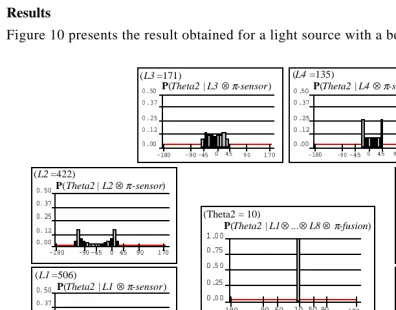
7.4 Results, lessons and comments
Results
Figure 10 presents the result obtained for a light source with a bearing of 10°:
The eight peripheral figures present the distributions
correspond-ing to the eight light sensors. The central schema presents the result of the fusion, the
distri-bution . Even poor information coming from each separate
sensor may blend as a certainty.
Sensor fusion method
In the experiment just presented, we have seen a simple instance of a general method to carry out data fusion.
The key point of this method is in the decomposition of the joint distribution, which has been considerably simplified under the hypothesis that «knowing the cause, the conse-quences are independent». This is a very strong hypothesis, although it may be assumed in
Figure 10: The result of a sensor fusion for a light source with a bearing of 10° l1t|l2t⊗…⊗l8t⊗π-fusion
( )
P
1
Σ
--- P(lit|Theta2⊗π-sensor)
i=1 8
∏
Theta2∑
× = 0.00 0.12 0.25 0.37 0.50-180 -90 -45 0 45 170
0 .00 0 .12 0 .25 0 .37 0 .50
-180 -90 -45 0 45 90 170
0.00 0. 12
0. 25
0. 37 0.50
-180 -90 -45 0 45 90 170
0.00 0.12
0.25
0.37 0.50
-180 -90 -45 0 45 90 170
0.00 0. 12 0. 25 0. 37
0.50
-180 -90 -45 0 45 90 170
0.00 0.12 0.25 0.37
0.50
-180 -90 -45 0 45 90 170
0.00 0.12 0.25 0.37 0.50
-180 -90 -45 0 45 90 170 0 .00 0 .12 0 .25 0 .37 0 .50
-180 -90 -45 0 45 90 170
0.0 0 0.25 0.5 0 0.75
1.0 0
-180 -90 -50 10 50 90 170
P(Theta2 | L3 ⊗π-sensor)
(L3 =171)
90
P(Theta2 | L4 ⊗π-sensor)
(L4 =135)
P(Theta2 | L5 ⊗π-sensor)
(L5 =280)
P(Theta2 | L6 ⊗π-sensor)
(L6 =489)
P(Theta2 | L2 ⊗π-sensor)
(L2 =422)
P(Theta2 | L1 ⊗π-sensor)
(L1 =506)
P(Theta2 | L8 ⊗π-sensor)
(L8 =511)
P(Theta2 | L7 ⊗π-sensor)
(L7 =511)
P(Theta2 | L1⊗ ...⊗ L8 ⊗π-fusion)
(Theta2 = 10)
Theta2|Li⊗π-sensor
( )
P
Theta2|l1t⊗…⊗l8t⊗π-fusion
( )
numerous cases.
This way of doing sensor fusion is very efficient. Its advantages are manifold. • The signal is heightened.
• It is robust to a malfunction of one of the sensors. • It provides precise information even with poor sensors. • It leads to simple and efficient computations.
In this experiment, another fundamental advantage of Bayesian programming is clearly evident. The description is neither a direct nor an inverse model. Mathematically, all vari-ables appearing in a joint distribution play exactly the same role. This is why any question may be asked of a description. Furthermore, there is none ill-posed problem. If a question may have several solutions, the probabilistic answer will simply have several peaks.
8. Hierarchical behavior composition
8.1 Goal and experimental protocol
In this experiment, we want to obtain phototaxy behavior based on and .
We have already built such behavior based on and , named .
How-ever, as we saw in the previous section (7), obtained by a sensor fusion has many
advantages on obtained by pretreatment.
8.2 Specification
Variables
The variables we require are the nine variables used in the sensor fusion description
and :
[S8.1]
Decomposition
The decomposition states that if we know , the position of the light source, then the
exact readings of the light sensors do not matter for :
[S8.2]
Parametric forms
The first distribution is directly obtained using the sensor fusion description:
Vrot Theta2
Vrot Theta1 π-phototaxy1
Theta2 Theta1
L1 L2 L3 L4 L5 L6 L7 L8 Theta2, , , , , , , , Vrot
L1∈{0, ,… 511}, L1 =512
…
L8∈{0, ,… 511}, L8 =512
Theta2∈{–170, ,… 180}, Theta2 =36 Vrot∈{–10, ,… 10}, Vrot =21
Theta2 Vrot
Theta2⊗L1⊗L2⊗L3⊗L4⊗L5⊗L6⊗L7⊗L8⊗Vrot|∆⊗π-phototaxy2
( )
P
Theta2⊗L1⊗L2⊗L3⊗L4⊗L5⊗L6⊗L7⊗L8|π-phototaxy2
( )
P ×P(Vrot|Theta2⊗π-phototaxy2)
[S8.3]
The second one is obtained from as:
[S8.4]
Specifications [S8.1], [S8.2], [S8.3] and [S8.4] are the components of preliminary knowledge .
8.3 Identification
No identification is required as there are no free parameters in .
8.4 Utilization
In order to drive Khepera toward the light with description , one should answer
the following question:
[E8.1]
Applying successively the marginalization rule ([E3.10]), the product rule ([E3.6]) and the specifications [S8.3] and [S8.4], we obtain:
[E8.2]
8.5 Results, lessons and comments
Results
The results obtained this way are presented in the three following figures.
Figure 11 presents the results for a light source in front of the robot. The left part shows
and the right part .
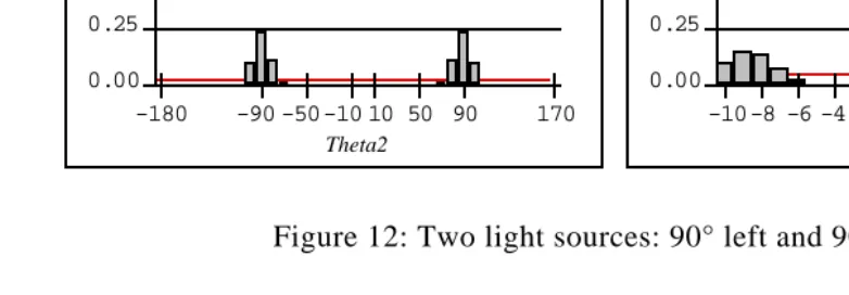
Figure 12 presents the results for two light sources, one 90° left of the robot, and the sec-ond 90° right. The left part exhibits two symmetrical peaks for . Consequently, the right part also shows two symmetrical
peaks for . The robot may decide to turn left or right with
equal probabilities.
If we suppose it decided to turn left, at next the time step Khepera will have the left light source 80° to its left and the right one 100° to its right. Figure 13 shows that it has then a high probability of continuing toward the left light source.
Hierarchical composition method
In Section 6 we showed a method of combining different behaviors (descriptions) in order to obtain more complex ones. By contrast, in this experiment we present a method to hierarchi-cally compose descriptions, in order to incrementally obtain more abstract ones.
Theta2⊗L1⊗L2⊗L3⊗L4⊗L5⊗L6⊗L7⊗L8|π-phototaxy2
( )
P
.≡P(Theta2⊗L1⊗L2⊗L3⊗L4⊗L5⊗L6⊗L7⊗L8|π-fusion) π-phototaxy1
Vrot|Theta2⊗π-phototaxy2
( )
P ≡P(Vrot|Theta2⊗π-phototaxy1)
π-phototaxy2
π-phototaxy2
π-phototaxy2
Vrot|l1t⊗…⊗l8t⊗π-phototaxy2
( )
P
Vrot|L1⊗…⊗L8⊗π-phototaxy2
( )
P
Vrot⊗Theta2|L1⊗…⊗L8⊗π-phototaxy2
( )
P Theta2
∑
=
Theta2|L1⊗…⊗L8⊗π-phototaxy2
( )
P ×P(Vrot|Theta2⊗π-phototaxy2)
Theta2
∑
=
Theta2|L1⊗…⊗L8⊗π-fusion
( )
P ×P(Vrot|Theta2⊗π-phototaxy1)
Theta2
∑
=
Theta2|L1⊗…⊗L8⊗π-fusion
( )
P P(Vrot|L1⊗…⊗L8⊗π-phototaxy2)
Theta2|L1⊗…⊗L8⊗π-fusion
( )
P
Vrot|L1⊗…⊗L8⊗π-phototaxy2
( )
A description of level may, thus, be used to infer a variable for a description at level
. In the experiment just described, for instance, the description is used to infer
for description , and the result of this hierarchical composition is the
description . In this experiment, all the information about is preserved. This
information is passed as the distribution and all the possible
values of are taken into account by way of the sum over this variable. However, as we
Figure 11: Light source in front of the robot.
Figure 12: Two light sources: 90° left and 90° right.
Figure 13: Two light sources: 80° left and 100° right.
0.00 0.25 0.50 0.75 1.00
-180 -90 -50-1010 50 90 170
0.00 0.25 0.50 0.75 1.00
-10 -8 -6 -4 -2 0 2 4 6 8 10
P(Theta2 | L1⊗ ...⊗ L8 ⊗π-fusion) P(Vrot | L1⊗ ...⊗ L8 ⊗π-phototaxy2)
Theta2 Vrot
0.00 0.25 0.50 0.75 1.00
-180 -90 -50-10 10 50 90 170
0.00 0.25 0.50 0.75 1.00
-10-8 -6 -4 -2 0 2 4 6 8 10
P(Theta2 | L1⊗ ...⊗ L8 ⊗π-fusion ) P(Vrot | L1⊗ ...⊗ L8 ⊗π-phototaxy2)
Theta2 Vrot
0.00 0.25 0.50 0.75 1.00
-180 -90 -50 -10 10 50 90 170
0.00 0.25 0.50 0.75 1.00
-10-8 -6 -4 -2 0 2 4 6 8 10
P(Theta2 | L1⊗ ...⊗ L8 ⊗π-fusion) P(Vrot | L1⊗ ...⊗ L8 ⊗π-phototaxy2 )
Theta2 Vrot
n
n+1 π-fusion
Theta2 π-phototaxy1
π-phototaxy2 Theta2
Theta2|L1⊗…⊗L8⊗π-fusion
( )
P
will show in 11, there is a possible alternative where a value for the variable at level is first
decided, then passed to the description at level . In our example, we could have drawn a
value for according to and then passed this value to
. This second method is obviously much more computationally efficient than the first one (the sum over is no longer necessary), although the price to pay is that some information is lost in this second process.
9. Situation recognition
9.1 Goal and experimental protocol
The goal of this experiment is to distinguish different objects from one another.
At the beginning of the experiment the robot does not know any object. It must incre-mentally build categories for the objects it encounters. When it knows of them, the robot must decide if a presented object enters in one of the categories or if it is something new. If it is a new object, the robot must create a new category and should start to learn it.
9.2 Specification
Variables
The Khepera does not use its camera for this task. It must «grope» for the object. It uses the «contour following» behavior to do so (see Figure 4). It does a tour of the presented object and computes at the end of this tour four new variables: the number of left turns, the number of right turns, the perimeter and the longest straight line. The values of these variables are not completely determined by the shape of the object, given that the contour following behavior is quite choppy.
We also require a variable to identify the different classes of object. The value is reserved for the class of unknown (not yet presented) objects.
Finally, we obtain:
[S9.1]
Decomposition
Obviously, the four variables , , and are not independent of one another.
How-ever, by reasoning similar to the sensor fusion case (see Section 7), we consider that knowing the object , they are independent. Indeed, if the object is known, its perimeter or the num-ber of turns necessary to complete a tour are also known. This leads to the following decom-position:
n n+1
Theta2 P(Theta2|L1⊗…⊗L8⊗π-fusion)
Vrot|Theta2⊗π-phototaxy1
( )
P
Theta2
n n
Nlt Nrt
Per Lrl
O O = 0
Nlt∈{0, ,… 24}, Nlt =25
Nrt∈{0, ,… 24}, Nrt =25 Per∈{0, ,… 9999}, Per =10000
Lrl∈{0, ,… 999}, Lrl =1000 O∈{0, ,… 15}, O =16
Nlt Nrt Per Lrl
[S9.2]
Parametric forms
We have no a priori information on the presented object:
[S9.3]
For an observed object ( ), we state that the distributions on and are Laplace
succession laws18 and that the distributions on and are Gaussian laws:
[S9.4]
Finally, we state that for a new object ( ) we have no a priori information about ,
, and :
[S9.5]
The preliminary knowledge composed of specifications [S9.1], [S9.2], [S9.3], [S9.4] and
[S9.5] is named .
9.3 Identification
When an object is presented to the robot, if it is recognized as a member of a class , the parameters of the two Laplace succession laws and the two Gaussian laws corresponding to this class are updated.
If the object is considered by Khepera to be a new one, then a new class is created and
the parameters of the distributions are initialized with the values of , , and just
read.
The learning process is incremental. Contrary to what we have seen up to this point, the identification and utilization phases are not separated. Each new experience changes the set
of data , and leads to a new description .
18. A Laplace succession law on a variable V is defined by: with the total number of observations,
the number of possible values for and the number of observations of the specific value . O⊗Nlt⊗Nrt⊗Per⊗Lrl|∆⊗π-object
( )
P
O|π-object
( )
P ×P(Nlt|O⊗ ⊗∆ π-object)×P(Nrt|O⊗ ⊗∆ π-object) =
.×P(Per|O⊗ ⊗∆ π-object)×P(Lrl|O⊗ ⊗∆ π-object)
O|π-object
( )
P ≡Uniform
O≠0 Nlt Nrt
Per Lrl
1+nv
N+ V
--- N
V V nv v
oi∈O ∀ ,oi≠o0 Nlt|oi⊗ ⊗∆ π-object
( )
P ≡L1(nNlt( )oi )
Nrt|oi⊗ ⊗∆ π-object
( )
P ≡L2(nNrt( )oi )
Per|oi⊗ ⊗∆ π-object
( )
P ≡G1(µ( ) σoi , ( )oi )
Lrl|oi⊗ ⊗∆ π-object
( )
P ≡G2(µ( ) σoi , ( )oi )
O = 0 Nlt
Nrt Per Lrl
Nlt|o0⊗π-object
( )
P ≡Uniform
Nrt|o0⊗π-object
( )
P ≡Uniform
Per|o0⊗π-object
( )
P ≡Uniform
Lrl|o0⊗π-object
( )
P ≡Uniform
π-object
oi
Nlt Nrt Per Lrl