© 2017 IJSRST | Volume 3 | Issue 8 | Print ISSN: 2395-6011 | Online ISSN: 2395-602X Themed Section: Scienceand Technology
A Comparative Analysis of Spatial Interpolation Incidence of Tuberculosis
Prevalence in Karnataka
Talluri Rameshwari K R
1, Rakshitha Rani N
2, Sunila
4, Ravi Kumar M
3and Sumana K
11,2Division of Microbiology and 3Division of Geo-informatics, Department of Water and Health, Faculty of Life
Sciences, JSS Academy of Higher Education and Research, Sri Shivarathreeshwara Nagar, Mysuru, India
4Department of Pathology, JSS Medical College and Hospital, JSS Academy of Higher Education and Research, Sri
Shivarathreeshwara Nagar, Mysuru, India
ABSTRACT
Tuberculosis is a bacterial air borne respiratory infectious disease caused by the Mycobacterium tuberculosis. Documented reports from 2011-16 by Revised National Tuberculosis Control Programme (RNTCP) revealed 26,628,020 Tuberculosis cases in India and 1,800,921 cases in Karnataka alone. The intensity of incidence, spread and the hotspots in Karnataka were focused using the tools of Geographical Information System (GIS), with comparative analytical procedure of spatial interpolation, cluster analysis and modeling the spatial pattern. It compares global and local indicators of spatial interpolation association for locating hotspot in spatial interpolation map. In the present study, Arc-GIS (Geographic Information System) interpolation tool is applied to identify the tuberculosis incidence hotspots in the Karnataka. Data for this study was obtained from the RNTCP. Statistical Package for the Social Sciences (SPSS) statistics revealed that the overall TB incidence in Karnataka is re-emerging from 2011-2016. The current study revealed the hotspots of TB incidence in Karnataka. The TB incidence in Bangalore, Belgaum, Mysore, Gulbarga and Raichur is recorded to be 18%, 21.78%, 11.88%, 11.66% and 22.1% respectively. Variation in incidence was observed during 2011-16, 28% incidence (2011-13), 1.765% decrease (2014-15) and 11.425% increase (2016), indicating re-emergence with more virulence and increased intonation pertaining to the incidence and spread. The present study is a novel concept with the intersection of GIS tool and the data analyzed targets the hotspots in these provinces, further, controlled management strategies may be intensified as remedial measures in the above geographical area.
Keywords : Tuberculosis Cases in Karnataka, Arc-GIS software (Demo Version), Spatial Interpolation, IDW method, Spatial Scan Statistics, SPSS Software for Statistical Graph.
I.
INTRODUCTION
Tuberculosis (TB) is a bacterial infectious disease caused by bacillus, Mycobacterium tuberculosis (M. tuberculosis). It is one among the world’s deadliest communicable diseases [1]. Since seventeenth century the pathological and anatomical illustration of M. tuberculosis appeared in human populations is still being a menace [2], World Health Organization (WHO) has declared TB a global health emergency in 1992 and it is reported to be prevalent in almost all countries of the world [3-4].
TB is a highly feared, known for centuries to affect the populations and continues to ravage the world and especially the developing country like India. It is spread through air by infectedpatients [5-6]
Pulmonary Tuberculosis sustains and spreads to other organs of the body. This is referred as Extra Pulmonary Tuberculosis. The lesions include the bronchus, lungs, pleura and intrathoracicbroncho pulmonary lymph nodes, bones and joints,Central Nervous System (CNS) (usually meningitis, but can occur in brain or spine),larynx, pericardial, abdominal sites; kidneys andgenitourinary tract. As the spread of the pathogen to different organs of the body, different proportion of spectrum of Extra Pulmonary Tuberculosis (EPTB) is noticed. The pathogen remains dormant for years at a particular site before causing the disease. The diagnosis at an early stage with proper epidemiological study improves focused diagnosis and administration [10].
managed to certain extent but has paved a threat by re-emerging over a period of time [7].
Statistical review of the Tuberculosis (TB) remains one of the leading infectious diseases throughout the world accounting for about 8.8 million (26%) cases in 2010 [8], among them 2.0 – 2.5 million cases is observed in India alone. WHO declared TB as re-emerging in 2011 and it is been a risk factor to mankind.
The incidence, spread and the hotspots, if traced, that area can be focused with more concern and the management strategies and module can be designed. This is the area of investigation in the current study, were the tools of Geographical Information System (GIS) and statistics favours in locating the spatial distribution, intensity of the incidence and hotspots at the province.
GIS - tools supports in finding the distribution of the TB cases and targeting the hotspot. Three tools of GIS helps in designing the graph that focuses on the distribution and hotspot of disease cases registered [9].
Arc-GIS software tool involves 3 types, viz.
ArcMap: The main mapping application, allows creating maps, querying attributes, analyzing spatial relationships and final projects layout.
ArcCatalog: Organizes spatial data contained in the computer and various other locations, it allows to access the search, preview and add data to ArcMap and also to manage metadata, finally setting up address locator services (geocoding).
ArcToolbox: Contains tools for geoprocessing, data conversion, coordinate systems, projections and etc. This workbook will focus on ArcMap and ArcCatalog.
ArcMap is made up of three software product levels
viz..ArcView, ArcEditor and ArcInfo. All these products share a common architecture but provide increasing levels of functionality. ArcView provides the base mapping and analysis tools. ArcEditor provides all ArcView capability and includes additional processing and advanced editing. ArcInfo provides all ArcEditor capability plus advanced analysis and processing [11, 12]
The technique recently available is Arc – GIS (Geographic Information System), where geographic data is used to describe and visualize spatial distributions. It also favours to discover spatial sodality patterns. Many studies encompasses the utility of GIS technology for spatial distribution of TB patients [13], socio-economic risk factors [14, 15], demographic risk factors [16], and TB transmission dynamics
in high-incidence areas [17]. In order to assess TB epidemiological situation nationwide, some studies used sizably voluminous data-set such as surveillance data [18] and National Health Indemnification data cognate with TB patients [18, 19]. GIS has additionally been utilized in coalescence with molecular epidemiological techniques to understand the dynamics of TB transmission [20, 21]. This technique is extrapolated for TB case studies currently for the study of incidence, spread and hotspots.
II.
METHODS AND MATERIAL
2.1 Tuberculosis Data Collection
The secondary data were collected from several organizations viz., TB registration data, demographic data, spatial data and Annual report of RNTCP [22].
This includes the confirmed TB cases notified from 2011-16. Report is based on the data collected annually from all Districts of Karnataka.
2.2 Arc- GIS Software 10.2.2 (Demo Version)
Interpolation is a procedure used to predict the values of cells at locations that lack sampled points. It is based on the principle of spatial autocorrelation or spatial
dependence that measures degree of
relationship/dependence between closer and distant objects.
Spatial autocorrelation determines the values correlated. If values are interrelated, it determines the spatial pattern. This correlation is used to measure similarities of objects within an area. This tool helps in creating the surface grid. Several
interpolation tools are exploited from spatial analyst extension.
The degree to which spatial phenomenon is correlated to itself in space.
The level of interdependence between the variables Nature and strength of the interdependence depends
on different interpolation methods that may produce different results.
Kriging - A statistical interpolation method used for diverse application such as health sciences, geochemistry, mapping and pollution modelling.
Spline - This estimates values using a mathematical function that minimizes overall surface curvature, this results in a smooth surface that passes exactly through the input points.
IDW - Inverse Distance Weight is one of the options of interpolation technique which estimates cell values of samples data points in the neighbourhood of each processing cell.
2.3 Spatial Auto Correlation Analysis
The caliber of spatial aggregation of TB patients in this study area by examining a spatial autocorrelation utilizing Ecumenical Moran’s I index statistics with row standardized inverse distance weights (IDW) matrices [23]. This method measures whether the values of neighbouring areas are similar to one another. Thus, the significant positive spatial autocorrelation implies that the distribution of TB patients is more spatially aggregated than a random underlying spatial process. The patient distributions were observed using Inverse Distance Weighted (IDW) interpolation with annual TB patient Incidence.
2.4 Hotspot Analysis
Activity space is spotted with statistical considerable local accumulation of TB patients.
The Getis-Ords has CT-level (Computed tomography) of hotspots and coldspots. Getis is detected with a spatial statistical method. Optimized hotspot analysis was done using Arc-GIS (Demo Version Software 10.2.2). Getis statistics is the ratio of the local sum of the values in the vicinity of a distance, in other words the scale of the analysis, to the sum of all values. When the local sum is different than the expected local sum and that difference is too astronomically immense to be the result of desultory chance, a statistical consequential Z-score is the result. The scale of analysis was tenacious through Spatial Autocorrelation (SA) [24, 25].
2.5 Spatial Pattern Detection
The TB Spatial pattern detections are divided into two types: Global detection and Local detection by SMRs
spatial patterns. These were accomplished using Arc-GIS 10.2.2 software (Demo Version).
2.5.1 Global Detection
Ecumenical detection technique was acclimated to examine the ecumenical pattern of TB occurrence. Spatial autocorrelation was acclimated to assess the degree of homogeneous attribute observed among a certain location and its neighboring units [25, 26]. Moran’s I coefficient was utilized as the speaker in this aspect. A weight matrix was accommodated to nominate a spatial relationships of the study area so that those that were imminent in space were given more weight in the calculations than those that were distinct [27].The TB infection is not a directional restricted because here the queen contiguity is utilized [26]. Moran’s I is an
extension of Pearson’s correlation coefficient to spatial neighbours. It gives a score ranging between -1 and 1. A score of zero designates the null hypothesis of no clustering. A positive score denotes clustering of areas of kindred attribute values, whereas a negative value designates that neighboring areas inclined to have dissimilar attribute values [26]. The paramountcy of Moran’s I was assessed utilizing Monte Carlo randomization. The calculations of statistical preeminence assess the consequence of the Moran’s I statistic opposes the null hypothesis [26, 27].
2.5.2 Local Detection
In the terms of spatial pattern detection of a TB disease, cluster analyses are paramount in order to detect aggregation of the disease cases, to test the occurrence of any statistically consequential clusters and ultimately to find evidence of etiologic factors. Cluster analysis identifies whether geographical aggregation of disease cases can be expounded by chance or be statistically consequential. In general, there are two types of spatial clustering methods, ecumenical and local ones. The ecumenical method is utilized to identify the presence of spatial clustering in the whole study area but does not designate location of the clusters. This circumscription is overcome by utilizing the local method which can pinpoint the characteristics of clusters in terms of their location, size, and magnitude [28, 26].
3 Statistical SPSS Analysis
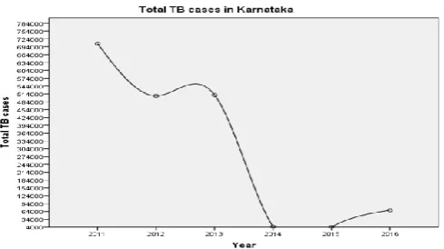
(SPSS), the Statistical analysis of TB incidence from 2011-16 in Karnataka and India overall curve is been designed in this study. SPSS analysis helps to determine about the relationship, outliers and graphically represent the relationship. In the current study the linear graph was generated out of the data from 2011-16. The variation of the incidence was noticed and statistically significant re –emergence of the incidence in 2016 was recorded.
III.
EQUATION
4.1. Incidence Rates Calculation and Adjustment Spatial autocorrelation is an evaluation of the connection of a variable in reference to spatial area of the variable, which is a match between area closeness and quality comparability [29]. The Spatial Autocorrelation device returns five esteems: The Moran's I Index, Expected Index, Variance, Z-score and P-esteem. Moran's I is the more prevalent test measurement for spatial autocorrelation. Worldwide Moran's I analyzes the spatial connection over a whole area and it is computed [30]:
Where N is the number of observations of the complete work field, range x2 and x1 are the observations at places of I and j, is the middle, half way between of X and w4 an part of spatial weights matrix, is the spatial
weight between places of i and j. The value of Moran’s I generally (make, become, be) difference between -1 and 1 [31].
The selection of neighbours is formally detailed in the weights matrix which makes picture of the relation between a part and its all round. A distance-based weight matrix was took up in this work-place and each distance part is detailed as a board forming floor of doorway distance, such that all places within the given distance are taken into account to be neighbours (the value not equal to zero in the matrix) in the distance-based weight matrix. A complete Moran’s I can be made regular to Z(I) and Z(I) is worked out as [30, 32]:
Where W1* is the addition of all weights placed in the noise, words i, W1* is the addition of all weights in the column i. The edge of 1.96 was sent in name for to test the sense, value level of Z (I). If Z (I) was greater than 1.96 or smaller than 1.96, suggests the importance of spatial autocorrelation [33].
The spatial correlogram is a graph where the Moran’s I makes line picture in ordinate against distances among places. In harmony with to Legendre and Fortin the spatial correlogram can be made regular into correlogram in which the ordinate is the made regular Moran’s I, Z (I) [34]. The form of the made regular correlogram provides ideas of about the spatial good example (spatial clusters and spatial outliers5) and spatial connection distance of Moran’s I which is not fixed in a level [34, 35]. However, the made regular correlogram often has one or more positive connection ranges [36].
Local Moran’s I is a nearby test numbers and facts for spatial autocorrelation, which is used to make out the places of spatial clusters and spatial outliers.
IV.
Results
5.1Potential Risk Factors of Tuberculosis Occurrences
The selection of the level of TB risk factors is important to determine the significant variable influence towards the local TB occurrences.
TB Case in India with Statistical Analysis
There were 26,628,020 TB incidence cases reported in the India since 2011-16. The incidence reported in 2011 was 7,550,522. It surged to the peak at 15,750,313in 2012. The incidences show a drastic decrease in 2013 with 59,058 cases. Then in 2014-15 shows 8,783,551 and 604,774 respectively. In 2016, the number of TB cases peaked to 1,754,957 (Fig. 1) by a SPSS graph and by Arc-GIS map we can notice the hotspot of the India (Fig. 2).
Figure 1: Overall Tuberculosis cases in India from 2011-16 by a SPSS graph.
Figure 2 : The overall Tuberculosis Incidence in India from 2011-16 by a IDW interpolation pattern with a
Quantile classify.
TB Case in Karnataka with Statistical Analysis
There were 1,800,921 TB incidence cases reported in Karnataka from 2011-16. The incidence reported from 2011-13 are 705,991, 506,483 & 509,305 respectively. The incidence decreased for two consecutive years at 5,839 and 4,751 cases in 2014 -15 respectively. In 2016, the number of TB cases is 68,552, a drastic increase. This shows the re-emergence of the TB in 2016 in Karnataka (Fig. 3).
5.2 Comparing Interpolation Methods
The TB incidence in Bangalore, Belgaum, Mysore, Gulbarga and Raichur is recorded to be 18%, 21.78%, 11.88%, 11.66% and 22.1% respectively (Fig. 4) with their respective population. Variation in incidence was observed during 2011-16. In 2011, 705991 (11%) cases were recorded. 2012 showed 506483 (8.44%), 2013 showed 509305 (8.488%), In 2014, 5839 (0.0973%), 2015, 4751 (0.0791%) and in 2016, 68552 (1.142%) indicating re-emergence with more virulence and increased intonation pertaining to the incidence and spread (Fig. 5).
Figure 4 :The overall Tuberculosis Incidence in Karnataka from 2011-16 by a IDW interpolation pattern with a Quantile classify.
Figure 7:Gestid-Ord (G) test of spatial autocorrelation of Tuberculosis Incidences
The Reported Tuberculosis cases 2011-2016
In 2011, 200,400, 47264 & 35397 cases were recorded in Bellary, Bangalore & Mysore respectively [Fig. 5 (A)] and 5,154 & 7,188 was observed in the Kodagu&Yadgiri. 45582, 36054 & 34,180 cases were recorded in Bangalore, Mysore & Belgaum respectively [Fig. 5 (B)] and 5,361 & 7,495 was observed in the Kodagu and Yadgiri during 2012. In 2013, 49,944 & 33,523 cases were noticed in Bangalore and Belgaum respectively [Fig. 5 (C)] and 5,256 cases in Kodagu. In 2014, 820 & 406 cases were recorded in Belgaum and Gulbarga respectively [Fig. 5 (D)] and only 23 cases in Ramanagar. In 2015, 661, 621 & 515 cases were recorded in the Bangalore, Udupi&Raichur [Fig. 5 (E)] districts. In 2016, the re-emergence of the TB was noticed, 9,424 & 528 cases were recorded in the Bangalore &Belagum respectively [Fig. 5 (F)] and 9,242 cases in Bangalore.
The number of cases in Karnataka showed the maximum, minimum and moderate registered cases at different time intervals (2011-16). The hotspot shows the increase in the TB incidence, in that particular area where we can straightly focus on that region to identify the TB Patients. There were a least number of cases in 2014-15 where it shows the decreases in TB cases due to medical processes or an attempt that was made by the public health division. In the 2016, TB cases were seen more which shows the re-emergence of TB in Karnataka.
5.3 Testing Global Measures for Spatial
Autocorrelation of Predicted Tuberculosis Incidence
The prediction enables us to further assess cluster analyses using global measures. In the global measures that is Moran’s I and Gestid-Ord were tested with the disaggregated data derived from the interpolation of TB prevalence. In this case, looking at it could be seen that the Moran’s I index has negative values -0.088876 (Fig. 6). This rejects the null hypothesis of no spatial autocorrelation and accepts the inverse perfect correlation. With this disaggregated data, the situation for Gestid-Ord G is also different from the previous analysis. The result has shown significant clusters with the Z score of -0.551180. There is however less than 1%
chance that the high clustered could be the result of random chance (Fig. 7).
5.4 Testing Global Measure for Spatial
Autocorrelation of Tuberculosis Incidence
This was the first step if the analyses aiming to initially detect the TB incidence. Annual values of the Moran’s I indices are presented in the current study.
Table 2: shows result of Global Moran’s I test across different periods. In all cases, the Moran’s I index depicted negative values which indicate negative spatial autocorrelation of the TB incidence. A further look at the p-value index (0.20 as the lowest recorded in all categories) also reveals that the neighbouring features have dissimilar characteristics as for the cluster to be considered statistically significant; the p-value for the feature must be small enough.
Table 3: presents results from the Gestid-Ord, general G as a global measure. Considering z and p-values which are the measures of statistical significance in this context, the interpretation of this result may not be uniform as in the case of Moran’s I. The year 2011 has recorded -0.753 and 0.451 for the z and p-value respectively. This suggests that low clustering of the TB incidence.
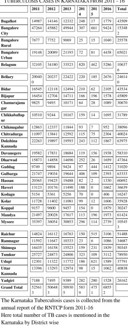
TABLE1
TUBERCULOSIS CASES IN KARNATAKA FROM 2011-16
2011 2012 2013 201 4
201 5
2016 Total
Bagalkot 14987 14146 12332 248 17 1779 43509 Bangalore
City
47264 45882 49944 307 661 9424 15348 2
Bangalore Rural
7677 7752 9069 25 15 1040 25578
Bangalore Urban
19148 20089 21193 72 81 4438 65021
Belagum 32105 34180 33523 820 462 5286 10637 6
Bellary 20040
0
20237 22422 220 185 2676 24614 0
Bidar 16545 12118 12494 210 62 2105 43534
Bijapur 16454 12704 14711 166 196 1578 45809 Chamarajana
gar
9825 9493 10171 64 28 1089 30670
Chikkaballap ur
10510 9244 10167 159 14 1695 31789
Chikmagalur 12863 12337 11844 93 7 952 38096 Chitradurga 11097 13841 12592 115 75 2304 40024 Dakshina
Kannada
22263 19897 19593 243 112 1867 63975
Davanegere 19582 17831 18684 119 156 1938 58310
Dharwad 15873 14858 14696 252 26 1659 47364
Gaddag 9749 9894 9424 97 444 1412 31020
Gulbarga 21747 19034 19644 406 109 2393 63333
Hassan 20365 19425 19488 82 2 1330 60692
Haveri 13123 10176 11490 188 0 1662 36639
Kodagu 5154 5361 5256 70 0 406 16247
Kolar 11728 11402 11081 99 12 1606 35928
Koppal 9157 9600 9457 154 0 1879 30247
Mandya 21497 20028 17617 113 196 1973 61424 Mysore 35397 36054 30853 296 114 2739 10545
3
Raichur 14824 16112 16763 150 515 3106 51488
Ramnagar 11592 11647 10333 23 6 1086 34687 Shimoga 16435 16158 15523 159 231 1839 50345
Tumkur 25727 24873 24806 323 109 3112 78950 Udupi 12301 11322 11772 186 621 1589 37791 Uttar
Kannada
13396 13293 12974 98 15 1062 40838
Yadgiri 7188 7495 9389 282 280 1528 26162
Grand Total 52561 3 50648 3 50930 5 583 9 475 1 6855 2
The Karnataka Tuberculosis cases is collected from the annual report of the RNTCP form 2011-16
Here total number of TB cases is mentioned in the Karnataka by District wise
G. Ord 2011 2012 2013 2014 2015 2016
Obser. G 0.031730 0.035006 0.034591 0.038495 0.037811 0.035476
Exp. G 0.035714 0.035714 0.035714 0.035714 0.035714 0.035714
Variance 0.000028 0.000003 0.000002 0.000011 0.000071 0.000003
Signf. (z)
-0.753121 -0.426078
-0.754755
0.831690 0.248474 -0.143581
P-Value 0.451377 0.670051 0.450396 0.405584 0.803768 0.885831
Table 3:Gestid-Ord (G)test for the spatial autocorrelation of Tuberculosis Incidences(2011-16)
Morani’s I
2011 2012 2013 2014 2015 2016
Moran’s I -0.058291 -0.107612 -0.155122
0.095991 0.053748 0.016407
Expected Index -0.035714 -0.035714 -0.035714 -0.035714 -0.035714 -0.035714
Variance 0.001901 0.017578 0.018172 0.012482 0.018251 0.015251
Z - Core
-0.517803 -0.542298
-0.885782
1.178835 0.662203 0.422059
P - Core 0.604596 0.587613 0.375735 0.238464 0.507841 0.672982
V.
Discussion
The research findings in the study were derived from the spatial pattern examination from Arc-GIS software (Demo Version) indicates the possible hot sites of the
TB in Karnataka. Using the maximum spatial cluster size for ≤ 50% of the total population, the spatial pattern analysis identified the most likely significant cluster for high occurrence of TB in Karnataka.
One of the main issues that emerge from this study is the reliability of global measures to test clustering pattern using collected secondary TB data. In the current study, overall Karnataka population is taken for calculating the percentage of TB cases in respective districts of Karnataka. From overall TB data in India out of 1,754,957 cases Karnataka shows 1,800,921 cases from the year 2011-16. In the present study the applicability of the measure of Moran’s I and Gestid-Ord is implemented where as in the study done by Mohammed Shahid et al. In their study sometimes it was based on the analysis of spatial autocorrelation index (high or low) [38, 39].
The hotspot of Karnataka is seen by the local spatial auto correlation which helps in the disease observation. That also explains the location of clusters as well as diversity of the TB patients in Karnataka [40]. It was found where these two methods local and global detection of the TB are involved in the study. This is in conformation with the studies conducted in England and Wales, Hong Kong, and Thailand [38, 39].
1. Variation in the Spatial Pattern Detection Techniques
The use of global measures to understand the spatial pattern through cluster detection has been widely acknowledged in health a science that is implemented in this study. Despite significant number of TB incidence in some of the unit areas in the study site, our analysis for spatial interpolation of the TB cases in Karnataka by year wise is remarkable. Contrastingly, our result (especially from the year 2011-16) has depicted to some level of the TB Quantile by using the IDW interpolation method. However, spatial methods which used mathematical models to predict the unknown using the
known points (interpolation) i.e. is to detect the TB hotspot in that particular area is one of the viable GIS techniques used to address data limitations [41, 42]. In other studies SiriwanHassarangseeet. al they have showed a Local Spatial Pattern and Spatial pattern detection of the TB in Thailand from 2004 – 2008 [38]. Such technique has been referred in the present study.
Particularly in this study the applicability of the measures Moran’s I and Gestid-Ord was done to the same study of the Sa’ad Ibrahim et. al in Nigeria. Whereas in Sa’ad Ibrahim et. al study the Moran’s I did not detect any clustering pattern for aggregated data. In their work-place, the use of such measures (Morans I and Gestid-Ord) was not quite successful using grouped facts. Sometimes the reasoned judgment based on the observations of spatial autocorrelation(high or low mass, group) could be misleading depending upon the index, the way of the knowledge and designing [43].
Regarding, our outcome especially for the year 2011-16 has represented some level of TB clustering pattern using the local and global detection. This contrasting study was done or conducted in the Karachi by
Muhammad Miandadet. al, Thailand by
SiriwanHassarangsee et. al, Nigeria by Sa’ad Ibrahim et. al, Tokiyo by Kiyohiko Izumi et. al, Nepal and Pakistan. [44, 45, 46, 47].
2. Limitations
Our study had some limiting conditions. Firstly, the study is conducted by the secondary data and demographic data which is collected in population rather than the individuals TB cases. Whereas this type of analysis can utilize the available data from the regular activities that also helps in the identification of the geographic map. Secondly, the study was taken for the period of 6 years i.e. from 2011-16 and additional data of the overall population adds the density to the TB cases in Karnataka that evaluates the spatial and interpolation trend of the TB pattern [49, 50].
VI.
CONCULSION
This study involves the use of GIS and spatial analyses which have been applied to many epidemiological researches to analyze and more clear display of spatial patterns of TB incidence in Karnataka.Like other developing states, the Karnataka is also one of the major TB causing states in India. For the first time the Arc-GIS method is used in the Tuberculosis incidence in Karnataka by the spatial interpolation model for predicting the TB prevalence employed in this study for identifying spatial pattern of TB. Prevalence has significant advantages and especially in the circumstances of poor data quality in which clustering data can be misleading or hard to reliably detect. This study has shown that despite data limitation, GIS approaches are quite viable for the understanding interpolation pattern. Thus, the outcome of this study is quite imperative for enhancing policy and decision making health service provision. The results of the study suggest that there was heterogeneity of spatial pattern of TB within the study region. The findings, in terms of the presence of hot spots of TB in this province, can help the provincial health officers to intensify the remedial measures in the identified areas and to issue future strategies for more effective control of this disease.
VII.
Acknowledgments
The authors are thankful to Ms. Chaithra for Statistical Graph analyses. We extend our gratitude to Jagadguru Sri Shivarathreeshwara University, Mysuru for the support.
VIII.
CONCLUSION
The proposed payment system combines the Iris recognition with the visual cryptography by which customer data privacy can be obtained and prevents theft through phishing attack [8]. This method provides best for legitimate user identification. This method can also be implemented in computers using external iris recognition devices.
IX.
REFERENCES
[1]. World Health Organization. Global Tuberculosis
Report 2014 [Internet]. 2014.
WHO/HTM/TB/2014.08
[2]. National Tuberculosis Center. Brief History of Tuberculosis. New Jersey: New Jersey Medical School; c1996 [Updated 1996 Jul 23]; [Cited 2009 Feb 26].
[3]. Anderson LF, Tamne S, Brown T, Watson JP, Mullarkey C, Zenner D, et al. Transmission of multidrugresistant tuberculosis in the UK: a cross-sectional molecular and epidemiological study of clustering and contact tracing. Lancet Infect Dis. 2014; 14: 406–15. doi: 10.1016/S1473-3099(14)70022-2PMID:24602842
[4]. World Health Organization: Highlights of activities from 1989 to 1998. World Health Forum1988; 9: 441-56
[5]. Murray M, Nardell E. Molecular epidemiology of tuberculosis: Achievements and challenges to current knowledge. Bull World Health Organ. 2002; 80: 477–482. PMID: 12132006
[6]. Munch Z, Van Lill SWP, Booysen CN, Zietsman HL, Enarson D a, Beyers N. Tuberculosis transmission patterns in a high-incidence area: a spatial analysis. Int J Tuberc Lung Dis. 2003; 7: 271–7.
[7]. Tiwari, N.; Adhikari, C.M.S.; Tewari, A.; Kandpal, V. Investigation of geo-spatial hotspots for the occurrence of tuberculosis in Almora district, India, using GIS and spatial scan statistic. Int. J. Health Geogr. 2006, 5. [CrossRef] [PubMed]
[9]. Couceiro, L.; Santana, P.; Nunes, C. Pulmonary tuberculosis and risk factors in Portugal: A spatial analysis. Int. J. Tuberc. Lung Dis. 2011, 15, 1445– 1454. [CrossRef] [PubMed]
[10]. Jones, S.G. & Kulldorff, M. 2012, "Influence of spatial resolution on space-time disease cluster detection", PLoS One, vol. 7, no. 10, pp. e48036. [11]. Chan-yeung M, Yeh a GO, Tam CM, Kam KM,
Leung CC, Yew WW, et al. Socio-demographic and geographic indicators and distribution of tuberculosis in Hong Kong: a spatial analysis. Int J Tuberc Lung Dis. 2005; 9: 1320–6.
[12]. Onozuka D, Hagihara A. Geographic prediction of tuberculosis clusters in Fukuoka, Japan, using the space-time scan statistic. BMC Infect Dis. 2007; 7. doi: 10.1186/1471-2334-7-26
[13]. SouzaWV, Carvalho MS, Albuquerque MDFPM, Barcellos CC, Ximenes R a a. Tuberculosis in intraurban settings: a Bayesian approach. Trop Med Int Heal. 2007; 12: 323–30. doi: 10.1111/j.1365-3156. 2006.01797.x
[14]. Maciel ELN, PanW, Dietze R, Peres RL, Vinhas SA, Ribeiro FK, et al. Spatial patterns of pulmonary tuberculosis incidence and their relationship to socio-economic status in Vitoria, Brazil. Int J Tuberc Lung Dis. 2010;
[15]. Alvarez-Hernández G, Lara-Valencia F, Reyes-Castro P a, Rascón-Pacheco R a. An analysis of spatial and socio-economic determinants of tuberculosis in Hermosillo, Mexico, 2000–2006. Int J Tuberc Lung Dis. 2010; 14: 708–13.
[16]. Barr RG, Diez-Roux A V., Knirsch CA, Pablos-Méndez A. Neighborhood poverty and the resurgence of tuberculosis in New York City, 1984–1992. Am J Public Health. 2001; 91: 1487– 93.
[17]. Feske ML, Teeter LD, Musser JM, Graviss EA. Including the third dimension: a spatial analysis of TB
[18]. cases in Houston Harris County. Tuberculosis.
2011; 91: S24–33. doi:
10.1016/j.tube.2011.10.006 PMID: 22094150 [19]. Tsai P-J. Spatial analysis of tuberculosis in four
main ethnic communities in Taiwan during 2005 to 2009. Open J Prev Med. 2011; 01: 125–134. doi: 10.4236/ojpm.2011.13017
[20]. Haase I, Olson S, Behr M a, Wanyeki I, Thibert L, Scott A, et al. Use of geographic and
genotyping tools to characterise tuberculosis transmission in Montreal. Int J Tuberc Lung Dis. 2007; 11: 632–8.
[21]. Moonan PK, Bayona M, Quitugua TN, Oppong J, Dunbar D, Jost KC, et al. Using GIS technology to identify areas of tuberculosis transmission and incidence. Int J Health Geogr. 2004; 3. doi: 10.1186/1476-072X-3-23
[22]. Bishai WR, Graham NMH, Harrington S, Pope DS, Hooper N, Astemborski J, et al. Molecular and geographic patterns of tuberculosis transmission after 15 years of directly observed therapy. J Am Med Assoc. 1998; 280: 1679–84. [23]. Moran PA. Notes on continuous stochastic
phenomena. Biometrika. 1950; 37: 17–23. Available:
http://www.ncbi.nlm.nih.gov/pubmed/15420245 PMID: 15420245
[24]. Getis A, Ord JK. The Analysis of Spatial Association. Geogr Anal. 1992; 24: 189–206. doi: 10.1111/j. 1538-4632.1992.tb00261.x
[25]. Ord JK, Getis A. Local Spatial Autocorrelation Statistics: Distributional Issues and an Application.
[26]. Geogr Anal. 1995; 27: 286–306. doi: 10.1111/j.1538-4632.1995.tb00912.x
[27]. Lai, P.C.; So, F.M.; Chan, K.W. Spatial Epidemiological Approaches in Disease Mapping and Analysis; CRC Press: New York, NY, USA, 2009.
[28]. Moran, P.A.P. Notes on continuous stochastic phenomena. Biometrika 1950, 37, 17–23. [CrossRef] [PubMed.}
[29]. Pfeiffer, D.U.; Robinson, T.P.; Stevenson, M.; Stevens, K.B.; Rogers, D.J.; Clements, A.C.A. Spatial Analysis in Epidemiology; Oxford University Press Inc.: New York, NY, USA, 2008. [30]. Cliff, A.D.; Ord, J.K. Spatial Autocorrelation;
Pion: London, UK, 1973; volume 178.
[31]. Cliff, A.D.; Ord, J.K. Spatial Processes: Models and Applications; Pion: London, UK, 1981. [32]. Overmars, K.P.; de Koning, G.H.J.; Veldkamp,
A. Spatial autocorrelation in multi-scale land use models. Ecol. Model. 2003, 164, 257–270.
[34]. Zhang, C.S.; McGrath, D. Geostatistical and GIS analyses on soil organic carbon concentrations in grassland of southeastern Ireland from two different periods. Geoderma 2004, 119, 261–275. [35]. Legendre, P.; Fortin, M.J. Spatial pattern and
ecological analysis. Plant Ecol. 1989, 80, 107– 138.
[36]. Zhang, C.S.; Tao, S.; Yuan, G.P.; Liu, S. Spatial autocorrelation analysis of trace element contents of soil in Tianjin plain area (in Chinese, with English abstract). Acta Pedol. Sin. 1995, 32, 50– 57.
[37]. Zhang, C.S.; Zhang, S.; He, J.B. Spatial distribution characteristics of heavy metals in the sediments of Changjiang River system—Spatial autocorrelation and fractal methods (in Chinese, with English abstract). Acta Geogr. Sin. 1998, 53, 87–96.
[38]. Anselin, L. Local indicators of association— LISA. Geogr. Anal. 1995, 27, 93–115
[39]. Julious, S.A.; Nicholl, J.; George, S. Why do we continue to use standardized mortality ratios for small area comparison? J. Public Health Med. 2001, 23, 40–46. [CrossRef] [PubMed]
[40]. Pickle, L.W.; White, A.A. Effects of the choice of age-adjustment method on maps of death rates. Stat. Med. 1995, 14, 615–627. [CrossRef] [PubMed]
[41]. Shannon, J. & Harvey, F. 2013, "Modifying areal interpolation techniques for analysis of data on food assistance benefits" in Advances in Spatial Data Handling Springer, pp. 125-141.
[42]. Faramnuayphol, P.; Chongsuvivatwong, V.; Pannarunothai, S. Geographical variation of mortality in Thailand. J. Med. Assoc. Thai. 2008, 91, 1455–1460. [PubMed]
[43]. Leung, C.C.; Yew, W.W.; Tam, C.M.; Chan, C.K.; Chang, K.C.; Law, W.S.; Wong, M.Y.; Au, K.F.
[44]. Socio-economic factors and tuberculosis: A district-based ecological analysis in Hong Kong. Int. J. Tuberc. Lung Dis. 2004, 8, 958–964. [PubMed]
[45]. Mangtani, P.; Jolley, D.J.; Watson, J.M.; Rodrigues, L.C. Socioeconomic deprivation and notification rates for tuberculosis in London during 1982–1991. BMJ 1995, 310, 963–966. [CrossRef] [PubMed]
[46]. Sasson, C.; Cudnik, M.T.; Nassel, A.; Semple, H.; Magid, D.J.; Sayre, M.; Keseg, D.; Haukoos, J.S.;Warden, C.R. Identifying high-risk geographic areas for cardiac arrest using three methods for clusteranalysis. Acad. Emerg. Med. 2012, 19, 139–146. [CrossRef] [PubMed]
[47]. Mansoer, J.R.; Kibuga, D.K.; Borgdorff, M.W. Altitude: A determinant for tuberculosis in Kenya? Int. J. Tuberc. Lung Dis. 1999, 3, 156– 161. [PubMed]
[48]. Vargas, M.H.; Furuya, M.E.Y.; Pérez-Guzmán, C. Effect of altitude on the frequency of pulmonary tuberculosis. Int. J. Tuberc. Lung Dis. 2004, 8, 1321–1324. [PubMed]
[49]. Vree, M.; Hoa, N.B.; Sy, D.N.; Co, N.V.; Cobelens, F.G.J.; Borgdorff, M.W. Low tuberculosis notification in mountainous Vietnam is not due to low case detection: A cross-sectional survey. BMC Infect. Dis. 2007, 7. [CrossRef] [PubMed]
[50]. Tanrikulu, A.C.; Acemoglu, H.; Palanci, Y.; Dagli, C.E. Tuberculosis in Turkey: High altitude and other socio-economic risk factors. Public Health 2008, 122, 613–619. [CrossRef] [PubMed] [51]. Kakchapati, S.; Yotthanoo, S.; Choonpradup, C.
Modeling tuberculosis incidence in Nepal. Asian Biomed. 2010, 4, 355–360.