Dynamic Analysis of a Three-dimensional Non-linear Continuous System

(1)

http://www.sciencepublishinggroup.com/j/pamj doi: 10.11648/j.pamj.20190802.12

ISSN: 2326-9790 (Print); ISSN: 2326-9812 (Online)

Dynamic Analysis of a Three-dimensional Non-linear

Continuous System

Abdellah Menasri

Department of Process Engineering, University of Constantine 3, Constantine, Algeria

Email address:

To cite this article:

Abdellah Menasri. Dynamic Analysis of a Three-dimensional Non-linear Continuous System. Pure and Applied Mathematics Journal. Vol. 8, No. 2, 2019, pp. 37-46. doi: 10.11648/j.pamj.20190802.12

Received: December 18, 2018; Accepted: March 19, 2019; Published: July 10, 2019

Abstract:

Most physical phenomena are modeled as continuous or discrete dynamic systems of a second dimension or more, but because of the multiplicity of bifurcation parameters and the large dimension, researchers have big problems for the study of this type of systems. For this reason, this article proposes a new method that facilitates the qualitative study of continuous dynamic systems of three dimensions in general and chaotic systems in particular, which contains many parameters of bifurcations. This method is based on projection on the plane and on an appropriate bifurcation parameter.

Keywords:

Dynamic Analysis, Nonlinear Continuous System, Three Dimensions

1 Introduction

The theory of chaos is one of the few, one of the very few mathematical theories that has had any real media success. It has even become a fashionable theory that it is fashionable to be able to cite if one wants to pass for someone cultured. We will even see that some of the great minds of this century quoted him without obviously knowing what they were talking about. Appeared in the early sixties in meteorology, it quickly spread to just about every science. Some have seen, or still see, a scientific revolution of equal importance to the appearance of Newton's mechanics, Einstein's relativity, or quantum mechanics.

The purpose of this article is to provide a new method for studying continuous three-dimensional dynamic systems with several bifurcation parameters [1]. This method gives important results on dynamic behavior, stability, bifurcations and chaos. This method has two steps, a projection on the plane to obtain a dynamic system of a smaller dimension, then the choice of the appropriate parameter. For simplicity, we consider a three-dimensional chaotic dynamic model with seven bifurcation parameters [2].

In this paper, a subsystem of the original system will be studied via an analysis of its dynamic behavior using a lower dimension (2D). This will be useful in the final study of the dynamic behavior of the original system.

2.

Dynamic Analysis of a Nonlinear

System in Three Dimensions

Consider the dynamic system defined by:

1

1 1 2 2 3 3

2 1 3 3

1 1 2 2 3

dx

a x a x a x dt

dx

x x b dt

dx

c x c x x c dt



= + +

 

= +

 

 ₌ ₊ ₊



(1)

Where, a_i≠0, (1≤ ≤i 3),c_i ≠0, (1≤ ≤i 2),b≠0and c≠0 are real parameters.

By the projection on the plane, (x₁−x₂)the following new system is obtained:

1

1 1 2 2 3 3

2 1 3

dx

a x a x a x dt

dx

x x b dt



= + +

   

= +



(2)

two-dimensional with constant coefficient. The Jacobian matrix of system (2) is:

1 2

3 0

a a J

x

 

= 

 

And, their determinant is given by:

det( )J = −a x_{2 3} For x₃≠0, we have det( )J ≠0 det(J)≠0. 2.1. The Fixed Point of the System (2)

The fixed point of the system (2) obtained from:

1 2 ₀

dx dx dt = dt = Hence

1 1 2 2 3 3 1 3

0

a x a x a x

x x b

+ + =

 

+ =

 (3)

With a simple calculation, the following is found

2

1 3 3

1 2

3 2 3

and

e b e a b a x

x x

x a x

−

= − =

Thus the system (2) has a single fixed point,

2 1 3 3 3 2 3

, a b a x

b x a x

e

_− − _

 

Using the translation:

1 1

2 2

e

x x x

y x x

 _{= −}  

= −



The point

e

can be reduced to the to the origin O.

2.2. Fixed Point Classification According to Eigenvalues

From the matrix J , we obtain:

2

1 2 3

det(λI−J)=λ −aλ−a x

We put

det(

λ

I− =J) 0

Hence

1 2 3

² a a x 0

λ

−

λ

− = (4)

Assuming that

,

a2 >0

1 For x₃>0, the equation (4) has two solutions

λ

₁ and

λ

₂ such that,

λ

1< <0

λ

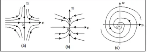
2 then the fixed point e is a "saddle" point. The curve of the solution in the plane

(

x1−x2

)

is represented in (Figure 1.a), where the directions of the orbits are represented by arrows when the time tincreases, when t tends to infinity only two orbits move towards the fixed point

e

, and the others diverge to infinity following two different directions.

2 For a1<0, when

2 1 3

2 4

a x

a

< − : The equation (4) has

two solutions

λ

1 and

λ

2 such that,

λ λ

1< 2<0, so, the fixed point

e

is a "Node", which explains the tendency of solution curves on the plane

(

x1−x2

)

to infinity with the exception of two orbits that tend towards point

e

. This is shown in (Figure 1.b), where the direction of the orbits is represented by arrows.

3 For a₁<0, when 2 1

3 2

0 4

a x a

− < < : The equation (4) has

two complex solutions conjugated with a negative real part, the fixed point

e

is a "focus". The curve of the solutions on the plane

(

x1−x2

)

is shown in (Figure 1.c), where the direction of the arrow is the direction of the orbit when the time t increases. When t tends to infinity, all the orbits move in spiral around to point

e

.

Figure 1. (a) the fixed point

e

is a saddle point, (b) The fixed point

e

is a "node", (c) the fixed point

e

is a "focus".

2.3. The Relationship Between the Time Variable t and the Function x t₃( )

When t tends to infinity, The orbit x t₃( )intersects the two

straight lines

2 1 3

2 4

a x

a

= − and x3=0alternately and several times. Hence, the division of the x₃ axis into three disjoint

domains 12 2 ,

4

a a

 

−∞ −

 

 

, 2 1 2

, 0 4

a a

 

−

 

 

and

(

0,+∞

)

Which implies the

possession of the system (2) of different dynamic behaviors in the three domains above. When tends to infinity the system (2) changes its dynamic behavior and x t₃( )passes through these domains repeatedly, leading to complex dynamics such as the appearance of bifurcations and chaos. It is noticed that the system (2) depends on time t when x t₃( )

varies over time. The two systems (1) and (2) can be verified that are chaotic when the function x t₃( )passes through the

straight lines

2 1 3

2 4

a x

a

(3)

2.4. The Fixed Point of the System (1)

Let us now look for the fixed point of the system (1), it results from the first and the second equation,

3 1

b x

x

= − (5) And

2 3 1 1 2

2 1

a b a x x

a x

−

= (6)

By substituting (5) and (6) into the third system equation (1), this equation is obtained,

3 2

2 1 1 ( 1 2 2)1 3 2 0

a c x + a bc +a c x −a c b= (7) To obtain a single fixed point, should be taken the case,

1 2

1 2 2

2 0 or a c

a bc a c c b

a

+ = = − (8)

Then, under the condition (8), the equation (7) has a unique real root,

3 2 3 1

2 1

a c

x b

a c

=

therefore the fixed point of system (1) is given by

2 3 2 3 1 1 3

2 1 2 1 1

, ,

a c a b a x b

E b

a c a x x

 ₋ 

−

 

 

2.5. Linearization of the System (2) at Fixed Point

(

1, 2, 3

)

E x x x

The stability of the equilibrium state (point E ), is analyzed by linearizing the system (1) to point E under the linear transformation,

1 0

2 0 3 0

x x x

y x y

z x z

= −

  ₌ ₋   ₌ ₋ 

Where

(9)

The system (1) becomes in the form:

1 2 3

0 0

1 2 0 2 0 2

dx

a x a y a z dt

dy

z x x z xz dt

dz

c x c z y c y z c yz dt



= + +

  

= + +

  

= + + +

 

(10)

The Jacobian matrix A E( )of the system (10) is

1 2 3

0 0

1 2 0 2 0

( ) 0

a a a

A E z x

c c z c y

 

 

=_ _

 

 

(11)

Its characteristic polynomial is given by

3 2

( )

P λ =λ +Aλ +Bλ+C (12) Where

2 0 1

2 3 1 1 2 0 2 0 2 1 0

( )

B bc a c a c y a z

A c y a

C a c x

= − +

 

= − + −

  ₌ 

(13)

Then, the conditions of Routh-Hurwitz lead to the condition that the real parts of the roots are λ -négative iff

0

A> , C >0 and AB− >C 0 . It is noticed that the coefficients of the polynomial (12) are all positive. So

( ) 0

P

λ

> for all λ>0. Therefore, the only fixed point is unstable ( rel( )

λ

>0 ), If P( )

λ

>0 has two conjugate complex eigenvalues. It is noticed that,

λ

₁=i

ω

and

2 i

λ

= −

ω

Since the sum of the three roots of the cubic P(λ) is

1 2 3

A

λ λ λ

+

= −

(14)

So, we have

λ

₃ = − =A c y_{2 0}+a₁which is located on the system stability margin (10).

From equality (14), we have

2

2 1 0 1 2 0 2 3 3

2 0

c a x a a x c a b a x

λ = − + + (15)

Then, we have

3

( ) 0

(4)

2 2

2 3 1 2 0 1 3 2 0 1 2 3 2 2 3 2

3 2 2 2

1 2 3 1 2 2 1 0 1 3 2 0 3 2 2 2 2 3 1 2 3 2

2 1 0

( ) ( )

a a c c x a a bc x a a a c b A

a a c b

a a a c c a c x a a bc x a bc a bc a a c B

a a c b C a c x

 ₊ ₋

=

 

 ₊ ₋ ₊ ₋



=

   ₌  

(17)

And

3 2 3 0

2 1

a c

x b

a c

=

A substitution of (17) in (16) and with a complicated computation, it is obtained

2 3 2 2 2 2 3 4 2 2 4 2

2 3 1 2 2 3 1 2 1 3 1 1 2 3 1 2 1 2 1 0

2 3 3 2 2 4 2 2 3 2 3 2

1 2 3 1 2 2 3 1 2 1 2 3 2 1 2 3 1 2 1 2 3 2 2 3 1 2 0

2 2 2 4 2 2 4 2 3 2 2 2 2 2

1 3 2 1 3 1 2 1 2 3 2 1 2 3 2 1 2 3

( )

a a bc c a a c c a a bc a a a c c a a c x

a a a bc c a a bc c a a a b c a a a bc c a a a bc a a bc c x

a a b c a a b c c a a a bc a a a b c a a a

− − − − +

− − + − + +

− + + − + bc c1 2=0

(18)

Or

3 2

1 1 1 0

a a a

α +β +γ + =δ (19) Where

4 2 2

3 1 0 2 3 2 0 2 2 2 2 4 2 3 1 2 0 3 2

4 2 2 3 2 4 2 2

2 1 0 2 3 1 2 2 3 2 2 3 1 2 0 2 2 4 2 3 2 2 2 2 2

3 1 2 2 3 2 2 3 2 2 3 1 2

2 3 2 2 2 2 2 3 2 3 2 2 3 1 2 2 3 1 2 0 2 3 1 2 2 3 1 2

( )

( ) ( )

a bc x a a bc x

a a c c x a b c

a c x a a bc c a a b c a a bc c x

a b c c a a bc a a b c a a bc c

a a bc c a a c c x a a bc c a a bc c x

α β γ δ

= − +

= − −

= − + − + −

+ + − +

= − + − + 0

        

(20)

Assume that, α >0and the equation (19) has a single solution a₁=a₀. Hence, for a₁=a₀the fixed point E will lose its stability, so a hopf bifurcation can occur. Using the two conditions (14), (16) and a1=a0. The polynomial P( )

λ

can be written in the form:

2 0 2 0

( ) ( )( )

P λ = λ−a −c y λ +Bɶ (21) Where

3 2 2 2

0 2 3 1 2 2 1 0 0 3 2 0 3 2 2 2 2 3 1 2 3 2

(a a a c c a c x) a a bc x a bc a bc( a a c )

B

a a c b

+ − + −

=

ɶ (22)

It is obvious that, the equation P( )

λ

=0 has three roots, one negative,

λ

3 =a0+c y2 0 and a pair of conjugated purely imaginary roots

3 2 2 2

0 2 3 1 2 2 1 0 0 3 2 0 3 2 2 2 2 3 1 1,2

2 3 2

(a a a c c a c x) a a bc x a bc a bc( a a c )

i id

a a c b

λ = ± + − + − = ± (23)

Differentiate the two sides of the equation P( )

λ

=0 for to a₁. We obtain

2 2

2 0 1 2 0 2 1 0

2 2

2

2 1

3 2

c x a bc x a c x

a a b

d

dt A B

λ λ

λ

λ λ

 

  ₋

− + 

  _ _

   

=

(5)

Hence

(

)

(

)

1 0

2 2

2 0 0 2 0 2 1 0

0 2 0

2 2

1 ₀ _{2 0}

2 1

Re 1

0 2

a a

d a c y

a a b

d

da _d _a _{c y}

λ

=

 

  ₋

− + +  

  _ _

   

= − <

+ + (25)

And

(

)

(

)

1 0

2

2 0 0 2 0 2 1 0

0 2 0

2 2

1 0 2 0

2 1

Im 1

2

a a

a c y

a a b

d

da _d _a _{c y}

λ

=

 

  ₋

− + + 

  _ _

   

= −

+ + (26)

Conclusion. 1

1 According to the Hopf bifurcation theorem, it can be concluded that a₀ is the critical value.

2 The fixed point E is stable, when a1<a0, and there are a periodic solutions when a₁>a₀.

3 When a1 crosses the value a0 , the system (1) undergoes a Hopf bifurcation at fixed point E.

3. Property of Hopf Bifurcation

In this section. The explicit formulas will be drawen to determine the orientation, stability and period of these periodic bifurcation solutions at point E for the critical value

1 0

a =a , using techniques of the normal form. 3.1. Supercritical and Subcritical Bifurcation

Let the eigenvectors corresponding to the eigenvalues

3 a0 c y2 0

λ

= + and

λ

₂ =idare v₁ and v₂+iv₃. By direct calculations, the following is obtained

2 2 1 0 0 2

2 2 2

1 0 2 0 0 2 2 2 0 0 3 2

2 2 2 2 2

2 1 0 2 0 3 2 2 2

0 2 0 2 3 2 0

2 2

0 2 0 3 0 2 3 2 2 2 2

2 2 0 3

2 2 2

2 2 1 2 0 0

2 2 2

2 0 2 0 0

1

( )

1

( )

(( ) ) ( )

a c x a a b

v a c x a a a bc x a a bc

a c a bc x a b c

a a x a a bc x

a a x a d x a a b

v a x a d

c b bc d c c x y

bc d x c dx y

 

 

−

 

₋ ₊ ₊ ₊ 

 

+ −

 

 ₋ 

 



− + −

+

− −

− +



2 2

3 2 0 3 1 0 3 1

2 2 2

3 2 3 2 3 1 0

2 2 2 2

1 2 1 0 2 0

2 2 2

2 0 2 0 0

0

( )

(( ) ) ( )

d a b c a a c x a bc v a a b c a c d x

c c b c d x c b y bc d x c dx y

           

 

 



 



 



 

 _ _



 



 



 



 

 _ _

 



 



 



 



 

 ₊ ₊

 



 ₊ 



 



 



 

 ₋ ₊

 

 _ _

− +

  



(27)

(6)

2

2 1 0 0 2 2 2 2 2

0 2 0 3 0 2 3 3 2 0 3 1 0 3 1

2 2 2

1 2 3 0 2 0 0 2 2 2 0 0 3 2 2 2 2 2 2 2 2

2 0 3 2 3 2 3 1 0

2 2 2 2 2 2 2 2

2 1 0 2 0 3 2 2 2 1 2

2 2

0 2 0 2 3 2 0 1

1 0

( )

( , , ) ( )

( ) ( )

a c x a a b

a a x a d x a a b d a b c a a c x a bc P v v v a c x a a a bc x a a bc

a x a d a a b c a c d x

a c a bc x a b c c b bc d c c x a a x a a bc x

− − + − + + = = − + + + + + + − − − −

2 2 2 2

0 0 1 2 1 0 2 0

2 2 2 2 2 2

2 0 2 0 0 2 0 2 0 0

( )

(( ) ) ( ) (( ) ) ( )

y c c b c d x c b y

bc d x c dx y bc d x c dx y

                 ₋ ₊     ₋ ₊ ₋ ₊    (28)

To facilitate the calculations, the matrix (28) is replaced by the following,

1 2 3

1 1 0

α α α β β β           (29) Where 2 2 1 0 0 2

1 2 2 2

0 2 0 0 2 2 2 0 0 3 2

2 2

0 2 0 3 0 2 3

2 2 2 2 2

2 0 3

2 2

3 2 0 3 1 0 3 1

3 2 2 2

2 3 2 3 1 0

( )

a c x a a b

a c x a a a bc x a a bc

a a x a d x a a b a x a d

d a b c a a c x a bc a a b c a c d x

α α α  ₋ =  − + + +   − + −  =  +   + +  ₌  ₊ 

2 2 2 2 2

2 1 0 2 0 3 2

1 _{2 2}

0 2 0 2 3 2 0

2 2 2

2 2 1 2 0 0

2 2 2 2

2 0 2 0 0

2 2 2 2

1 2 1 0 2 0

3 2 2 2

2 0 2 0 0

( )

(( ) ) ( )

( )

(( ) ) ( )

a c a bc x a b c a a x a a bc x

c b bc d c c x y

bc d x c dx y

c c b c d x c b y

bc d x c dx y

β β β  ₊ ₋ =  −   − −  =  − +   − +  ₌  ₋ ₊  (30)

Then, perform the following transformation on the system (10) 1 2 3 u x

y P u

z u         =             Hence 1 1 2 3 u x

u P y

z u −         =            

In order to obtain

1 1 2 3

2 1 2 3

3 1 2 3

u m x m y m z

u n x n y n z

u k x k y k z

= + +   = + +   ₌ ₊ ₊  (31) Therefore 1

2 1 2 3

2

1 1 2 3

3

3 1 2 3

( , , )

du

du F u u u dt

du

du G u u u dt

du

u H u u u dt λ  = − +    = +    = +   (32) Where

1 2 3 2 1 2 3 3 2 1 2 3

1 2 3 1 2 1 1 2 2 3 3

1 2 3 1 1 2 2 3 3 1 1 2 2

F(u ,u ,u ) = m f(u ,u ,u )+ m c g(u ,u ,u ) G(u ,u ,u ) = n f(u ,u ,u )+ n c g(u ,u ,u ) H(u ,u ,u ) = k f(u ,u ,u )+ k c g(u ,u ,u )

f(u ,u ,u ) = (u + u )( u + u + u ) g(u ,u ,u ) = ( u + u + u )( u + u +

β β β

α α α β β β3 3u )        

1 3 3 1 1

3 3 2 1

3 2

3 3 2 1

3 3

3 3 2 1

1 ( )( ) ( )( ) ( )( ) m m m α β α β β α α α β β α α α α β α α α   ₋  = +    − −     = −  − −   = −  − − 

3 1 1 3 1

3 2 1 3 2 1

3 2

3 2 1 3 2 1

3 3

3 2 1 3 2 1

( ) ( ) ( ) ( ) ( ) ( ) n n n α β α β β α α α β β β β α α α β β α β α α α β β  ₋ =  − − −   =  − − −   = −  − − − 

1 2 2 1 1

3 2 1 3 2 1

1 2

2

3 2 1 3 2 1

2 1

3

3 2 1 3 2 1

( ) ( ) ( ) ( ) ( ) ( ) k k k α β α β β α α α β β β β β α α α β β α α β α α α β β  ₋ =  − − −   ₋  =  − − −   ₋ = −  − − − 

Applying now, the method of Auchmuty and Nicolas (Hasard and al.1981, Zhang, 1991), from system (32), the following quantities can be calculated at a₁=a₀ and

(0, 0, 0)

(7)

2 2 2 2

11 ₂ ₂ ₂ ₂

1 2 1 2

1

4

F

G

g

i

u



∂



∂



=



+



+



∂



∂







Hence

(

)

(

)

(

)

11 2 1 2 2 3 2 1 1 3 2 2 2 2 1 2 2 3 2 1 1 3 2 2 2

1 1

2 2

g = m β +mβ +m c α β +m cα β + i n β +n β +n cα β +n cα β

And

2 2 2 2 2 2

02 ₂ ₂ ₂ ₂

1 2 1 2

1

2 2

4

F F G G G F

g i

u u u u

u u u u

 

∂ ∂ ∂ ∂ ∂ ∂

= − − + _ − + _

∂ ∂ ∂ ∂

∂ ∂ ∂ ∂ 

Hence

(

)

(

)

02 2 1 2 3 2 1 1 2 2 2 1 2 3 2 2 1 1 2

2 1 2 3 2 1 1 2 2 2 1 2 3 2 2 1 1 2

1

( ( ) ( ) ( )

2 1

( ) ( ) ( ) ( )

2

g m m c n n c

i n n c m m c

β β α β α β β β α β α β

= − + − − + − + +

− + − + + + +

On the other hand

2 2 2 2 2 2

20 ₂ ₂ ₂ ₂

1 2 1 2

1

2 2

4

F F G G G F

g i

u u u u

u u u u

_∂ _∂ _∂ _∂ _∂ _∂ 

 

= _ − + + _ − − __

∂ ∂ ∂ ∂

∂ ∂ ∂ ∂ 

 

Therefore

(

)

(

)

20 2 1 2 3 2 1 1 2 2 2 1 2 3 2 2 1 1 2

2 1 2 3 2 1 1 2 2 2 1 2 3 2 2 1 1 2

1

( ( ) ( ) ( )

2 1

( ) ( ) ( ) ( )

2

g m m c m m c

i n n c m m c

β β α β α β β β α β α β

= − + − − + + + +

− + − − + − +

And

3 3 3 3 3 3 3 3

21 ₃ ₂ ₂ ₃ ₃ ₂ ₂ ₃

1 1 2 1 2 2 1 1 2 1 2 2

1 8

F F G G G G F F

G i

u u u u u u u u u u u u

_∂ _∂ _∂ _∂ _∂ _∂ _∂ _∂ 

 

= _ + + + + _ + − − __

∂ ∂ ∂ ∂ ∂ ∂ ∂ ∂ ∂ ∂ ∂ ∂ 

 

Therefore

21 0

G =

In addition to

2 2

11 ₂ ₂

1 2

1 4

H H

h

u u

_∂ _∂ 

= _ + _

∂ ∂

 

Hence

(

)

11 2 1 2 3 2 1 1 2 2

1

( ) ( )

2

h = k β β+ +k c α β α β+

And

2 2 2

20 ₂ ₂

1 2

1

2 4

H H H

h i

u u

u u

_∂ _∂ _∂ 

= _ − − _

∂ ∂

 

Therefore

(

)

(

)

(

)

20 2 1 2 3 2 1 1 2 2 2 1 2 3 2 2 1 1 2

1

(

)

(

)

(

)

2

h

=

k

β β

−

+

k c

α β α β

−

i k

β β

+

k c

α β α β

+

(8)

1 11 11

1 20 20

( 2 )

h

id h

λ ω

= −

 

− = −

 (33)

The solution of the system (33) is

11 11

1 20 20

1

( 2 )

h

h id

ω λ ω

λ



= −

    _{= −}

 ₋



Hence

(

)

(

)

(

)

(

)

2 1 2 3 2 1 1 2 2 11

1

2 1 1 2 3 2 1 1 2 2 2 1 2 3 2 2 1 1 2

20 2 2

1

2 1 2 3 2 1 1 2 2 1 2 1 2 3 2 2 1 1 2 2 2

1

( ) ( )

2

( ) ( ) 2 ( ) ( )

2( 4 )

2 ( ) ( ) ( ) ( )

2( 4 )

k k c

k k c d k k c

d

d k k c k k c

i

d

β β α β α β

ω

λ

λ β β α β α β β β α β α β

ω

λ

β β α β α β λ β β α β α β

λ

 ₊ ₊ ₊

= −

 

 ₋ ₊ ₋ ₊ ₊ ₊ ₊



= − +



+



 ₋ ₊ ₋ ₋ ₊ ₊ ₊



 ₊



On the other hand, we have

2 2 2 2

110

1 3 2 3 1 3 2 3

1 2

F G G F

G i

u u u u u u u u

 _∂ _∂  _∂ _∂ 

= _ ₊ ₊ _ ₋ __

∂ ∂ ∂ ∂ ∂ ∂ ∂ ∂ 

 

Therefore

(

)

(

)

(

)

(

)

(

)

(

)

(

)

(

)

110 3 2 2 3 2 3 1 3 2 2 3 3 1 3 2

3 2 2 3 2 3 1 3 2 2 3 3 1 3 2

1 2 1 2

G m n c m n c m n

i n m c n m c n m

β α β β β α α

= + + + + + +

− + − + −

Then

(

)

21 21 2 110 11 110 20

g =G + G ω +G ω

Hence

(

)

(

)

(

)

(

)

(

)

(

)

(

)

(

)

(

)

(

)

21 3 2 2 3 2 3 1 3 2 2 3 3 1 3 2

2 1 2 3 2 1 1 2 2

1

3 2 2 3 2 3 1 3 2 2 3 3 1 3 2

2 1 1 2 3 2 1 1 1 2 2 2 1 2 3 2

2 2

1

3 2 2 3 2 3 1 3

( ) ( )

2

1 4

( ) ( ) 2 ( )

2( 4 )

1 4

g m n c m n c m n

k k c

m n c m n c m n

k k c d k k c

d

m n c n m

β β α β α β λ

λ β β λ α β α β β β

λ

β α β

= + + + + + ×

 ₊ ₊ ₊ 

− −

 

 

− + − + − ×

 ₋ ₊ ₋ ₊ ₊ ₊ 

−

 

 ₊ 

 

+ +

(

+

)

(

)

(

)

(

)

(

)

(

)

(

)

(

)

(

)

(

)

(

)

2 2 3 3 1 3 2

2 1 2 3 2 1 1 2 2 1 2 1 2 3 2 2 1 1 2

2 2

1

3 2 2 3 2 3 1 3 2 2 3 3 1 3 2

2 1 2 3 2 1 1 2 2 1 2 1 2 3 2 2 1 1 2

2 2

1

2 ( ) ( ) ( ) ( )

2( 4 )

1 4

2 ( ) ( ) ( ) ( )

2( 4 )

c n m

d k k c k k c

d

i m n c m n c m n

d k k c k k c

d

β β α α

λ

+ + ×

 ₋ ₊ ₋ ₋ ₊ ₊ ₊ 

+

 

 ₊ 

 

− + − + − ×

 ₊ ₊ ₋ ₋ ₊ ₊ ₊ 

 ₊



(

)

(

)

(

)

(

)

(

)

(

)

3 2 2 3 2 3 1 3 2 2 3 3 1 3 2

1 2 1 2 3 2 1 1 2 2 2 1 2 3 2

2 2

1 1

4

( ) ( ) 2 ( )

4

i m n c n m c n m

k k c d k k c

d

λ β β α β α β β β

λ

+

 

+ + + + + ×

 ₋ ₊ ₋ ₊ ₊ ₊ 

−

 

 ₊ 

(9)

Finally, we have

2 2

1 20 11 11 02 21

1 1 1

(0) 2

2 3 2

C g g g g g

d

 

=  − − +

 

(

1

)

2

0 Re (0) Re( '( ))

C a

µ = − _λ

1 2 0

2

Im(C(0)) ( '(a ))

d

µ λ

τ

= − +

2 2 Re(C1(0))

γ

=

We know that

1.

µ

2 Determines the direction of the Hopf bifurcation. i If >0, the Hopf bifurcation is subcritical.

ii If _µ₂<0, the Hopf bifurcation is supercritical and the bifurcated periodic solution exists for

a

₁

>

a

₀and

0 1

a

<

.

2.

γ

₂ Determines the bifurcated periodic solution stability.

i If _γ₂<0, the bifurcated periodic solutions on the central collector are stable.

ii If _γ₂ >0, the bifurcated periodic solutions on the central collector are unstable.

3. τ₂ Determines the periods of the bifurcation of the periodic solutions.

i If _τ₂>0, the periods increase. ii If _τ₂<0, the periods decrease. 3.2. Numerical Simulation

The numerical simulation confirms the results obtained by this method

For

a

₂

=

1

.

5

, a

₃

=

2

, b=

−

1

.

3

, c=

−

1

.

5

and

c=

−

1

. 1. If a₁=−1.221.

The attractor generated by the chaotic system (1) as shown in (Figure 2).

Figure 2. The chaotic attractor for the system (1).

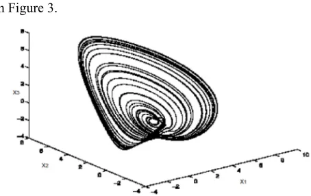
2. If a1=−1.440.

The attractor generated by the chaotic system (1) as shown

in Figure 3.

Figure 3. The chaotic attractor for the system (1).

4. Conclusion

In this paper, a three - dimensional quadratic system with seven bifurcation parameters has been studied. Using a projection on the plane and choosing a suitable bifurcation parameter, this method has been proved that can help us to simplify the study of bifurcations and in particular the Hopf bifurcation, have been demonstrated that it occurs when the bifurcation parameter a1 crosses the critical value

a

₀. The direction of the Hopf bifurcation and the stability of the bifurcated periodic solutions are analyzed in detail.

References

[1] J. Lu, T. Zhou, G. Chen & S. Zhang, [2001] "Local bifurcations of the Chen system", International Journal of bifurcations and Chaos, 12, 2257-2270.

[2] T. Zhou & G. Chen, [2006] "Classification of Chaos in 3-D Autonomous quadratic System-I", International Journal of Bifurcation and Chaos, 16, 2459--2479.

[3] S. Dadras, H. Re. Momeni & Qi. Guoyuan, [2007] "Analysis of a new 3-D smooth autonomous system with different wing chaotic attractors and transient chaos", Indian Journal of Microbiology, 62, 391-405.

[4] B. K. Maheshwari, K. Z. Truman, [2004] 3-D finite element nonlinear dynamic analysis for soil-pile-structure interaction, 13th World Conference on Earthquake Engineering Vancouver, B. C., Canada, 1570.

[5] Paulo B. Gonçalves, Frederico M. A. Silva, Zenn J. G. N. Del Prado, [2016] Reduced order models for the nonlinear dynamic analysis of shells, 19, 118-125.

[6] Dejan Zupan, [2018] Dynamic analysis of geometrically non-linear three-dimensional beams under moving mass, Journal of Sound and Vibration, 413, 354-367.

[7] Jihua Dong, [2016] A dynamic systems theory approach to development of listening strategy use and listening performance, Elsevier, 63, 149-165.

(10)

[9] Liqiang Yao, Weihai Zhang, [2018] Stability analysis of random nonlinear systems with time-varying delay and its application, Journal of latex classe files.

[10] Marwen Kermani, Anis Sakly, [2019] On Robust Stability Analysis of Uncertain Discrete-Time Switched Nonlinear Systems with Time Varying Delays, Mathematical Problems in Engineering, 2018, 14.

[11] Màrio Bessa, Jorge Rocha, Paulo Varandas, [2018] Uniform hyperbolicity revisited: index of periodic points and equidimensional cycles, Journal dynamical systems, 33, 4. [12] Stephen Baigent, Zhanyuan Hou, [2017] Global stability of

discrete-time competitive population models, Journal of Difference Equations and Applications, 23, 8.

[13] S. O. Papkov, [2016] Three-Dimensional Dynamic Problem of the Theory of Elasticity for a Parallelepiped, Journal of Mathematical Sciences, 215, 2, 121-142.

[14] Xianmai Chen, Xiangyun Deng, Lei Xu, [2018] A Three-Dimensional Dynamic Model for Railway Vehicle--Track Interactions, Journal of Computational and Nonlinear Dynamics, 13, 7, 1-10.