CU splitting early termination based on weighted SVM

R E S E A R C H

Open Access

CU splitting early termination based on weighted

SVM

Xiaolin Shen

and Lu Yu

Abstract

High efficiency video coding (HEVC) is the latest video coding standard that has been developed by JCT-VC. It employs plenty of efficient coding algorithms (e.g., highly flexible quad-tree coding block partitioning), and outperforms H.264/AVC by 35–43% bitrate reduction. However, it imposes enormous computational complexity on encoder due to the optimization processing in the efficient coding tools, especially the rate distortion optimization on coding unit (CU), prediction unit, and transform unit. In this article, we propose a CU splitting early termination algorithm to reduce the heavy computational burden on encoder. CU splitting is modeled as a binary classification problem, on which a support vector machine (SVM) is applied. In order to reduce the impact of outliers as well as to maintain the RD performance while a misclassification occurs, RD loss due to misclassification is introduced as weights in SVM training. Efficient and representative features are extracted and optimized by a wrapper approach to eliminate dependency on video content as well as on encoding configurations. Experimental results show that the proposed algorithm can achieve about 44.7% complexity reduction on average with only 1.35% BD-rate increase under the“random access”configuration, and 41.9% time saving with 1.66% BD-rate increase under the “low delay”setting, compared with the HEVC reference software.

Keywords:HEVC, fast coding unit decision, classification, SVM, feature selection.

1. Introduction

High definition (HD) and ultra-high definition (UHD) video contents have become increasingly popular world-wide, thus the demand of video compression technologies that can provide higher coding efficiency over HD/UHD videos can be envisioned in near future. In view of this, high efficiency video coding (HEVC) standard is being developed by the Joint Collaborative Team on Video Co-ding [1], which is established by the ITU-T Video CoCo-ding Experts Group and the ISO/IEC Moving Picture Experts Group. HEVC outperforms H.264/AVC high profile by 35–43% bitrate reduction at the same reconstructed video quality [2]. HEVC inherits the well-known block-based hy-brid coding scheme [3] used by previous coding standards, e.g., H.264/AVC, and extends the framework by introdu-cing highly flexible quad-tree coding block partitioning. The quad-tree coding block partitioning consists of newly brought concepts of coding unit (CU), prediction unit

(PU), and transform unit (TU). CU is the basic unit of region splitting used for inter/intra coding, which extends the traditional concept of macroblock (MB) based on a hierarchical structure with block size varying from 64 × 64 to 8 × 8 pixels. A CU is allowed to recursively be split into four smaller CUs of equal size. In this manner, a picture is represented by a content-adaptive coding tree structure comprised of CU blocks with different sizes. PU is the basic unit used for prediction process in a rectangular shape. One PU can be encoded with one of the modes in candidate set, which is similar to MB mode of H.264/AVC in spirit. The pixels in one PU share prediction informa-tion, e.g., modes, motion vectors (MV), and reference index. TU is the basic unit for transform and quantization. TU is defined in a similar way as CU, and its size varies from 4 × 4 to 32 × 32. As reported in [4,5], the flexible data structure representation (extending the MB size up to 64 × 64) introduced over 10% bitrate saving in compari-son with the 16 × 16-based configuration in H.264/AVC, since the flexibility of block partitioning can effectively deal with the diversity of picture content.

* Correspondence:[email protected]

1_{Institute of Information and Communication Engineering, Zhejiang}

University, Hangzhou, China

2_{Zhejiang Provincial Key Laboratory of Information Network Technology,}

Hangzhou, China

However, the flexibility of block partitioning of HEVC imposes significant computational burden on encoder during seeking of the optimal combinations of CU, PU, and TU sizes. Thus, it is crucial for practical implemen-tation of the new standard to reduce the complexity while maintaining the coding performance. Researches on accelerating the encoder of HEVC test model (HM) are emerging. A fast intra mode decision algorithm [6] was proposed, which made use of the direction informa-tion of the neighboring blocks to reduce the number of directions taking part in rate distortion optimization (RDO) process. To reduce the computational complexity of TU size selection, a fast algorithm for residual quad-tree mode decision was proposed in [7]. Besides, the depth-first decision process for TU size selection in HM was replaced by a merge-and-split decision process, which also reduces unnecessary computation by using the inheritance property of zero-blocks and early ter-mination schemes for non-zero blocks.

In this article, we focus on CU size selection for HEVC. A content-based fast CU decision algorithm was deve-loped for HEVC TMuC (test model under consideration) [8], which analyzed the ratio of utilized CUs to total num-ber of CUs in different depth in frame level and skipped the rarely used CUs with specified depths. Information of neighboring and co-located CUs was used to skip CUs in unnecessary depth in CU level. The algorithm investiga-ted temporal and spatial correlations of CU depth, and designed different thresholds to control the number of CU depths to be evaluated. However, the correlations were data dependent and the ratio was affected by enco-ding configurations, such as the hierarchical depth in hie-rarchical prediction structure. Spatial correlation of CU depth as well as the probability that neighboring CUs were SKIP mode was considered in [9] to design an adaptive weighting factor, which was used to adjust the threshold in early terminating the following RD calculations of the current CU. In [10], a method for complexity controlling was proposed by limiting the number of coding decision tests and comparisons according to temporal correlations. All these related works explored the spatial correlations and/or temporal correlations of CU depth to eliminate specific CU depths with a trivial impact on RD perfor-mance. However, they were not robust enough due to di-versity of the content. It is necessary to consider more statistics so as to get a more accurate and stable model to simplify the CU splitting.

In the field of accelerating the encoder of H.264/AVC as well as its extensions, various properties were investi-gated and employed to simplify mode decision. A nearly sufficient condition for early zero-block detection is con-structed based on the analysis of prediction error to speed up the motion estimation of H.264/AVC JM refe-rence software in [11]. It indicated that prediction error

offered a valuable clue about encoder acceleration. Spa-tial and temporal correlations were exploited to predict the skip mode [12] to reduce encoder complexity. In [13,14], distribution of MV in an MB was chosen as a feature to predict the optimal mode other than perfor-ming exhaustive search over all modes. A hierarchical algorithm proposed in [15] categorized all type of modes into three levels which were triggered on by evaluating SAD (which is between current MB and its co-located MB), high-frequency energy in DCT domain, and RD cost of mode P-8 × 8. In [16], a fast mode decision algo-rithm named motion activity-based mode decision was proposed. It classified MBs into different classes by pre-defined thresholds and motion activity. Each class co-rresponded to different number of modes to be checked. Tiesong et al. [17] projected encoding modes onto a 2D map and an optimal 2D map was predicted using spatial and temporal information. Then, a priority-based mode candidate list was constructed based on the optimal 2D map and mode decision was performed starting with the most important mode in the candidate list with early ter-mination conditions. In such a way, the number of modes to be evaluated was reduced and acceleration was achieved. Changsung and Kuo [18] presented a feature-based fast inter/intra mode decision algorithm. This algorithm computed three features regarding spatial and temporal correlations with which to determine inter or intra mode to use. The feature space were partitioned into three regions, i.e., free, tolerable, and risk-intolerable regions by checking the RD loss due to wrong mode decision and the probability distribution of inter/intra modes. Depending on the region, mechan-isms with different complexity were applied for final mode decision. Martinez-Enriquze et al. [19] analyzed the conditional pdfs for every mode and estimated the RD cost to decide the optimal mode. A fast stereo video encoding algorithm based on hierarchical two-stage neural network was proposed in [20]. Local properties of input data and predicted error were extracted as the input feature to train a neural network which was designed to predict the optimal partition mode. SVM were also introduced in the study of fast mode decision [21,22]. However, MBs were treated equally in the classi-fication problem, and the RD performance of an MB was ignored. In general, these works exploited various mode-related features to predict the optimal mode or reduce the number of modes to be evaluated. The fea-tures included spatial and temporal correlations, the gra-dient or high-frequency energy, the RD cost of specific mode, motion activity, and local properties, such as the prediction error or SAD/sum of absolute transformed differences (SATD).

time-consuming for practical implementation, which will be further analyzed in Section 2. To solve this problem, we propose a method utilizing machine learning to accelerate the CU size selection process. With properly modeling the problem and applying machine learning algorithm, our method can accurately predict the opti-mal decision on CU splitting instead of exhaustive searching over all possibilities. In order to derive a more accurate model to predict the CU splitting decision, RD difference is introduced as weights in the SVM training procedure to alleviate the RD performance degradation due to misclassification. Furthermore, various features are extracted from input video as well as earlier encoded data and an optimal feature subset is derived by a wra-pper feature selection algorithm.

The rest of the article is organized as follows. We briefly go through CU size selection process of HM, and present the motivation of the proposed algorithm in Section 2. In Section 3, we elaborate the modeling of the CU splitting problem and its solution based on a machine learning algorithm, i.e., SVM. Experimental results in Section 4 demonstrate the effectiveness of the proposed algorithm, and Section 5 concludes the article.

2. CU size optimization in HM

To adapt to the diversity of picture content, flexible quad-tree coding block partitioning is adopted into HEVC which enables the use of CU, PU, and TU. The concept of CU is analogous to MB in pervious stan-dards, e.g., H.264/AVC. It is the basic unit for intra/inter coding and is always square in shape. Pictures are divided into many largest CUs (LCUs), and each LCU

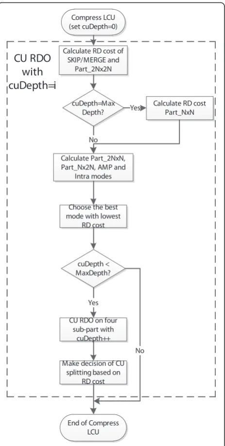
can be splitting into four equal-sized CUs which can be further recursively split up to the maximal allowable hierarchical depth. In such a manner, the LCU is con-structed as a quad-tree of CU(s) with different size as it shown in Figure 1. At leaf node of the quad-tree, the CU can be encoded in SKIP, inter, or intra mode. The parti-tioning size of SKIP mode is 2N× 2N, which means that the PU size of SKIP mode equals to CU size; the CU encoded in inter mode can be treated as one PU or par-titioned into several PUs, which is specified by partition-ing mode: Part_2N × 2N, Part_2N × N, Part_N × 2N, (Part_N ×N), Part_2N ×nU, Part_2N× nD, Part_nL × 2N, and Part_nR × 2N; and the CU in intra mode can be treated as one PU with size of 2N × 2N, or partitioned into four N× NPUs. A simple example of PUs in one CU is shown in Figure 1, as highlighted by the green square. PU corresponding to different partition size is the basic unit to carry the prediction information. In order to match the boundaries of real objects in a pic-ture, the shape of PU is not restricted to being square, e.g., 2N×Nis allowed. TU is defined for the transform and quantization process. The shape of TU depends on PU. When PU is square, TU is also square and its size varies from 4 × 4 to 32 × 32 luma samples. When PU is non-square, TU is also non-square and takes a size of 32 × 8, 8 × 32, 16 × 4, or 4 × 16 luma samples. One CU may contain one or more PUs. As well one CU may contain one or more TUs which are arranged in quad-tree structure as shown in Figure 1.

As explained in the previous paragraph, one LCU can be coded into a rather complex quad-tree to adapt to various video contents. Furthermore, CUs with different

depths may be coded in different prediction modes, di-fferent partitioning modes, and didi-fferent transform sizes. To derive the optimal CU-level coding parameters, an exhaustive search method is employed by evaluating the RD costs of all possible combinations of CU size, PU size, and TU size. The RDO of CU size is illustrated in Figure 2. It needs a total of 85 RD calculations when CU size varies from 64 × 64 to 8 × 8. Obviously, such RD-based optimization method introduces significant complexity on encoder. Actually, it is unnecessary to do an exhaustive search over all possible CU sizes, since there exist some CU sizes that do not result in much rate distortion improvement and it is possible to

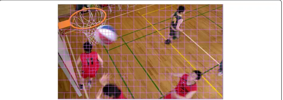
ac-celerate the encoder by early terminating the CU spli-tting decision process. As shown in Figure 3, “flat” or

“homogenous” regions, e.g., the floor, are more likely to be encoded in large CUs. Areas containing moving objects or objects boundaries, e.g., the net and the bas-ketball, are usually split into small CUs. Motivated by this observation, we model CU splitting decision as a binary classification problem.

3.CU splitting early termination algorithm based on weighted SVM

3.1. Problem formulation

As the flexible representation of coding data introduces heavy burden on the encoder, we propose to early ter-minate CU splitting to avoid unnecessary trials. We model CU splitting as a binary classification problem, (i.e., a CU that is not split into four sub-parts is assigned a label +1, otherwise−1 is assigned,) and tackle the clas-sification problem by SVM [23]. As a widely used ma-chine learning algorithm, SVM is based on the idea of structural risk minimization (SRM) and it has success-fully been applied to a number of real-world problems, such as face recognition, text categorization, and object detection in machine vision. The main idea behind SVM is to derive a unique separating hyperplane that maxi-mizes margin between two classes. Given ltraining data points

xi;yi

f gl

i¼1;xi∈RN;yi∈f1;1g: ð1Þ where {xi,yi} is the ith training sample, i.e.,ith CU. xiis

the input feature vector andyiis the class label indicating

CU splitting or not. The membership decision rule is based on the function defined in Equation (2), wheref(x) represents the discriminant function associated with the hyperplane.

f xð Þ ¼wTϕð Þ þx b: ð2Þ

where ϕ(·) is a nonlinear operator that maps the inputxi

into a higher-dimensional space and it is the kernel function.

Mathematically, this hyperplane can be constructed by minimizing the following cost function

J wð Þ ¼1

2w T_w¼1

2w

2_¼Xl

i¼1

w2i: ð3Þ

with constraints

yi wT:φð Þ þxi b

≥1: ð4Þ

For a non-separable case, the classification problem is generalized by introducing slack variables ξi and a

defined regularization parameterC. Then the classification problem is to minimize the following quantity

J wð Þ ¼1

2w

T_wþCXl

i¼1

ξi: ð5Þ

subject to

yiðwTφð Þ þxi bÞ≥1ξi

ξi≥0 :

ð6Þ

The modified cost function in Equation (5) is the so-called structural risk, which balances the empirical risk (i.e., the training errors reflected by the second term) with model complexity (the first term) [24]. It has been proven that the solution to the optimization prob-lem of Equation (5) under the constraint of Equation (6) is given by the saddle point of Lagrange function

Γðw;b;α;ξ;βÞ ¼1

2w

2_þ

CX

l

i¼1

ξi

Xl i¼1

αi yi wTφð Þ þxi b

1þξ_i

Xl i¼1

β_iξi:

ð7Þ

whereαiand βiare Lagrange multipliers associated with

the constraints in Equation (6).

The Lagrange multipliers are solved as maximizing

α _¼argmax α

Xl

i¼1

αi 1 2

Xl

i¼1

Xl

j¼1

αiαjyiyjK xi;xj

: ð8Þ

subject to

Xl

i¼1

αiyi¼0; C≥αi≥0; i¼1;2;. . .;l: ð9Þ

where K(xi, x) = φT(xi)φ(x). The decision function can

equivalently be expressed as

signðf xð ÞÞ ¼sign X l

i¼1

α

iyiK xð i;xÞ þb

!

: ð10Þ

It is obvious from Equation (10) that theαi associated

with training point xi expresses the strength with which

that point is embedded in the final decision function. Notice that the nonlinear mapping ϕ(·) never appears explicitly in the training or the decision. In general, the kernel takes the form of linear, polynomial, radial basis function (RBF), or sigmoid. In this article, we use the RBF kernel, since it can handle the case when the relation between class labels and the input vector is nonlinear as well as linear. Furthermore, the model complexity of the RBF kernel is lower than polynomial, and RBF kernel has fewer numerical difficulties [25].

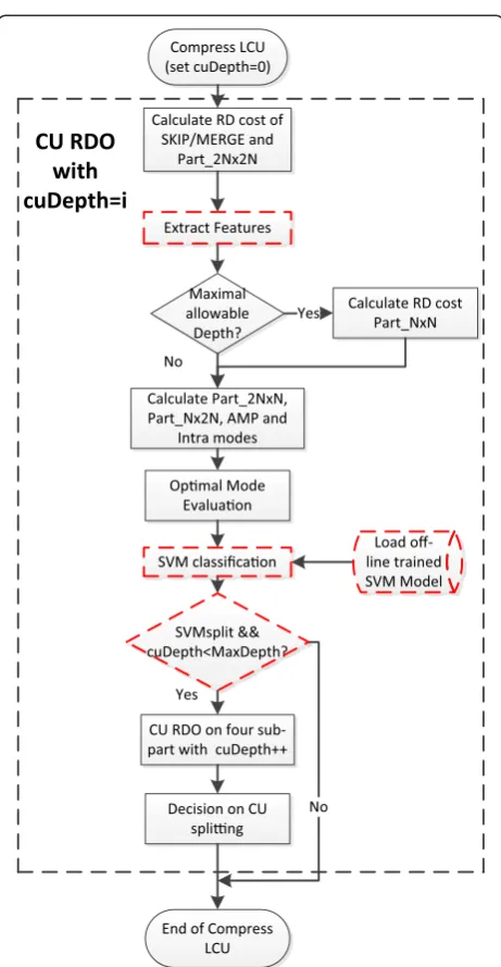
3.2. Proposed CU splitting early termination algorithm

The off-line trained SVM model is optimized based on SVM procedure with weighting on training samples. The weights are proposed as the difference of RD costs due to misclassifications. It is obvious that as long as the CU splitting predictor is accurate, early terminating RD trials on CU splitting can reduce a lot of computational com-plexity while maintaining RD performance.

3.3. CU splitting early termination algorithm based on weighted SVM

3.3.1. Off-line training and weights generation

In the field of machine learning, accuracy is one of the most important measurements for classification algo-rithms. However, in this scenario, not only the ratio of

correct classification, but also the loss of RD performance introduced by misclassifications is important.

There exist some CUs that the RD cost difference between four sub-CUs coding and one CU coding are almost the same. Misclassification of such CUs results in negligible RD degradation. On the contrary, for CUs that four sub-CUs coding outperforms one CU coding greatly, misclassification does lead to much RD loss. Obviously, different CUs are of different importance. It is improper to treat samples with different RD perfor-mance equally in the training process, and the optimal hyperplane will be deviated by those“unimportant” sam-ples, i.e., these samples are outliers. The desired SVM predictor should predict class label as accurate as pos-sible and keep RD loss as low as pospos-sible. Based on this observation, we suggest introducing weights into the SVM training process, i.e., assigning different weights to training samples.

xi;yi;Wi

f gl

i¼1;xi∈RN;yi∈f1;1g;Wi∈R: ð11Þ where the weights are defined as the percentage of RD cost increased due to misclassification, which is

Wi¼Ci s

ð Þ Cið Þn Cið Þn ;

when the CU is actually encoded in one CU

Wi¼Ci n

ð Þ Cið Þs

Cið Þs ; otherwise 8

> > < > > :

ð12Þ

where Ci(s) and Ci(n) are RD cost of splitting the CU

into four sub-CUs and RD cost of non-splitting CU, respectively. CU with little difference of RD cost is assigned a small weight, while CU with large difference of RD cost is assigned a large weight. Note that the weights are only needed in the training procedure, and not needed anymore when the trained model is used to predict the class label in the encoding process.

Then the standard SVM optimization problem in Equation (5) becomes

J wð Þ ¼1

2w

T_wþCXl

i¼1

ξiWi: ð13Þ

and the solution of the problem is

α_¼argmax α

Xl

i¼1

αi

1 2

Xl

i¼1

Xl

j¼1

αiαjyiyjK xi;xj

:

ð14Þ Figure 4Proposed CU early termination algorithm based on

subject to

Xl

i¼1

αiyi¼0; CWi≥αi≥0; i¼1;2;. . .;l: ð15Þ

The upper bounds of αi are bounded by dynamical

boundariesC*Wiinstead of a constant valueC. Then the

CUs with larger difference when encoded into one CU and into four sub-CUs will affect the optimal hyperplane more by introducing a larger weightWi.

3.3.2. Feature selection

We introduce several representative features related to CU splitting. Selecting effective and relevant features is crucial for classification. Good features help reduce training time as well as utilization time, defy the curse of dimensionality to improve prediction performance, and reduce storage requirements [26]. To select the features that are useful to build a good predictor of SVM, there are usually two types of feature selection approaches, fil-ters and wrapper approaches. In this article, we suggest using a wrapper method based on F-score [27]. Filter methods based on correlation or mutual information ranking [21] are easy to implement; however, selecting the most relevant variables is usually suboptimal for building a predictor, particularly if the variables are redundant. Wrapper method assesses a subset of fea-tures according to their usefulness to a given predictor, which is better in this scenario. However, the number of subsets is extremely large as the number of features increase, and thus exhaustive search is not proper. Therefore, we propose to rank all features first by

F-score and perform a greedy search based on the ranked results. F-score, as define in Equation (16), is a simple metric that measures the discrimination of two sets of real numbers.

F ið Þ≡ x ― i

þ

x ― i

ð Þ2_þ

x ―

i ―xi

ð Þ2

1 nþ1

Xnþ

k¼1

xþ_k;i―x_iþ

2

þ 1

n1 Xn

k¼1

x_k;i―x_i

2:

ð16Þ

where x―i ;x―i þ;x―i : are the average of the ith feature of the input vectorx of the whole, positive, and negative training samples, respectively.xk,i+is theith feature of the kth positive sample and xk,i− is the ith feature of the kth

negative sample.n+andn− are the total numbers of posi-tive and negaposi-tive training samples. The larger theF-score is, the more likely this feature is more discriminative.

F-score is easy to calculate and is friendly to be coupled

with SVM training process. The procedure of the wrapper approach is summarized in the following four steps:

(1) Collect training samples by running the HEVC reference software HM6.0.

(2) CalculateF-score of every feature in the training set and sort the features in descending order according to F-score.

(3) Start from one feature formed subset F (only one feature with the highest F-score).

(a) Randomly divide the training set intoStrandScv.

(b) Train SVM model using theStr.

(c) PredictScvand get the cross validation (CV)

(based on accuracy rate).

(d) Add the feature with the highestF-score in the rest to subsetFand repeat steps in (3) until all features are evaluated or early terminate this process by defining the maximum feature number.

4) Find the optimal feature subset with the lowest validation error.

To setup a rich feature set, diverse features are intro-duced and evaluated. Furthermore, it is possible to elimi-nate the dependency on video content by considering as many features as possible and then optimizing the feature subset. The features we consider as potential candidates are summarized as follows.

Prediction error-related features, such as SATD and CBF, denoted asxstd,xvrs, andxcbf.xstdis defined as

the SATD between prediction and original pixel values, andxvrsis the variance of four SATDs of

sub-block.xcbfis the coded block flags (CBF) of the

inter 2N× 2Nmode. CBF indicates the complexity of the predicted error under specific quantization parameters (QP). As discussed in [11-15], these features are correlated with CU partitioning.

CU depth information of the context [8], denoted as xsl,xsa, andxtp.xslandxsaare the CU depth of

left-neighboring and above-left-neighboring CU,

respectively.xtpis the CU depth of the co-located

CU. Since there is substantial correlation in spatial and temporal domain of video signal, such context provides very good information.

Gradient magnitude of current CU [18], denoted as xgm. It is the summation of gradient of every pixel in

the current CU by applying Sobel operator, which reveals the flatness of the CU.

Motion consistency-related feature [13,14], denoted asxmc, which is defined as the variance of the MVs

with inconsistent motion activities are more likely to be encoded in small CUs.

RD cost difference between skip and inter 2N× 2N mode, denotes asxdrc. If the skip mode is better

than inter 2N× 2N, the CU is likely to be

background and it maybe not necessary to partition the CU into smaller ones. On the contrary, if inter 2N× 2Nmode is better, it may be better to apply smaller partition mode or smaller CU size.

Side information in RD cost, denotes asxsi. Small

size motion partition provides good RD performance for those blocks with high motion activities or rich in content. However, more bits should be paid to signal the side information. Therefore, the

percentages of side information in total RD cost of inter 2N× 2Nmode give good indication of optimal CU size.

Hierarchical structure-related feature, denotes as xhrc. For the hierarchical prediction structure in

HEVC, small CU size is preferred for frames with low temporal depth and large CU size is more likely to be optimal for the frames with high temporal depth.

All the above-mentioned candidate features are eva-luated and an effective feature subset is formed by the proposed wrapper approach based on F-score. The experimental results on feature selection are presented. Although some of the features are correlated, the wra-pper method can select the useful feature to the pre-dictor regardless of correlation, as discussed in [26]. The video sequences we use in feature selection are“Cactus”,

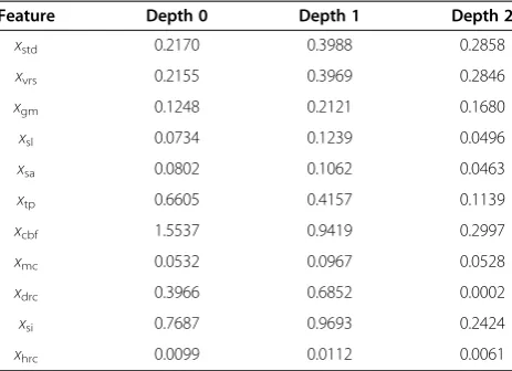
“BQMall”, and “FourPeople” and the training samples are collected by running HM6.0 [28] under common test conditions. In Table 1, it presents the F-scores of diffe-rent features in diffediffe-rent CU depths. CBF information

xcbf and side information in RD cost xsi exhibit relative high F-score and give good information about CU spli-tting. In contrast, the F-score of xhrc is rather low and therefore is excluded from the input vector in the fea-ture selection. Table 2 presents the feafea-ture subsets in selection procedure and its corresponding CV. The CV is nearly the same when feature number is greater than five. However, it takes more time to extract the features and the SVM predictor will become more complex as the number of features raises. It is a good choice to set the feature number as five, as shown in Table 2, consid-ering the balance between accuracy and additional com-plexity introduced by feature extraction and SVM model predictor. The optimized feature subsets are [xcbf, xsi,

xtp, xdrc, xstd], [xcbf, xsi, xtp, xdrc, xstd], and [xcbf, xsi, xtp,

xgm, xstd] for CU depth zero (CU 64 × 64), one (CU 32 × 32), and two (CU 16 × 16), respectively. Since the op-timal feature subsets are different for different CU

depths, the proposed CU splitting early termination models are trained separately for different CU depths. The overhead introduced by feature extraction is almost negligible, since most of them can be derived when cal-culating the RD cost of Skip and inter 2N× 2Nmodes.

4. Experimental results

4.1. Experimental results on the proposed CU splitting early termination algorithm

To verify the efficiency of the proposed CU splitting early termination algorithm, we conduct comprehensive experiments by comparing the proposed algorithm with HEVC reference software HM6.0. The encoding confi-guration exactly follows what is recommended in [29] and the test sequences in the experiments cover a variety of content. The sequences we use to train the SVM pre-dictor model are “Cactus”, “BQMall”, and “FourPeople”, denoted as TS1 (training set 1) and they are not used in performance comparison anymore. The offline training process is carried out by the SVM training software [30] and the proposed CU early termination algorithm is incorporated into HEVC reference software HM6.0.

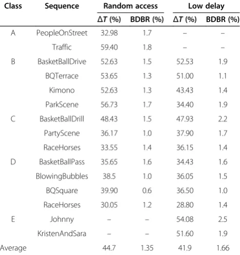
To evaluate the performance of the proposed algo-rithm, two metrics are used in Tables 3 and 4: the ave-rage BD-rate (BDBR) [31] difference between the proposed algorithm and HM6.0, and the time reduction ratio which is defined as

ΔT ¼THMTp

THM

100%: ð17Þ

whereTHMandTpare the total encoding time of HM6.0

encoder and the proposed encoder, respectively. The actual encoding time is measured on a workstation with a 2.93-GHz processor and 8 GB of RAM. In Tables 3 and 4, we present the RD performance and the compu-tational complexity of the proposed algorithm and the Table 1F-score of features in different CU depth

Feature Depth 0 Depth 1 Depth 2

xstd 0.2170 0.3988 0.2858

xvrs 0.2155 0.3969 0.2846

xgm 0.1248 0.2121 0.1680

xsl 0.0734 0.1239 0.0496

xsa 0.0802 0.1062 0.0463

xtp 0.6605 0.4157 0.1139

xcbf 1.5537 0.9419 0.2997

xmc 0.0532 0.0967 0.0528

xdrc 0.3966 0.6852 0.0002

xsi 0.7687 0.9693 0.2424

anchor under “Random Access, main” and “Low Delay, main”configurations.

Regarding complexity, the proposed algorithm achieves a maximum of 73.7% running-time reduction with respect to HM6.0 with an average of 44.7% under“Random Ac-cess, main”configuration, as shown in Tables 3 and 4. In Table 3, the column of “ΔT” is the average ΔT of 4 QP points. Concerning the RD performance, it loses 1.35% in terms of BD-rate on average, and a worst case of 1.8% for sequence“Traffic”. The RD loss is not significant. For the

“Low Delay, main”configuration as shown in Tables 3 and 4, the proposed algorithm behaves very similar to the

“Random Access, main”case and it reduces the complex-ity by 41.9% with 1.66% RD-Rate loss on average. In Table 4, part of the experimental results under different QPs is listed. As can be seen from it, more complexity re-duction is achieved in low bitrate scenario (i.e., using high QP values). In such cases, larger CUs are more efficient in RD performance than smaller CUs, and large CUs take a high percentage. The proposed algorithm accurately early

terminates the RDO procedures on large CU size and avoids unnecessary RD calculations on small CU size. Therefore, greater complexity reduction can be achieved in low bitrate case than the high bitrate case.

To verify that different training set will not affect the per-formance of the proposed algorithm, additional experiment is conducted. Three different sequences (“ParkScene”,

“BasketballDrill”, and“Johnny”, denoted as TS2) are used to train the offline model which is to be used in the encod-ing process. The encodencod-ing configurations are the same as the previous experiments. The metrics used in Table 5 are the same with that in Table 3. As shown in Table 5, similar RD performance and complexity reduction are derived using a different training set.

Both the weighted SVM training algorithm and the wrapper feature selection algorithm have been designed to provide the ability to generalize. First of all, the weighted SVM is based on SRM principle as opposed to traditional empirical risk minimization principle employed by con-ventional learning algorithms. SRM minimizes an upper bound on the expected risk, which equips the SVM with great ability to generalize. Introducing RD difference as weights eliminates the influence of outliers. In other words, those training samples with little RD performance degradation due to misclassification are“almost excluded” by assigning small weights and more attention is paid to

“important” samples. Second, large number of relevant features are evaluated and assessed. Diversity of features lowers the opportunity of dependence on training set. The Table 2 CV of different feature subsets

Input feature X1 X2 X3 X4 X5 X6 X7 X8 X9 X10

Depth 0 CV [xcbf] [X1,xsi] [X2,xtp] [X3,xdrc] [X4,xstd] [X5,xvrs] [X6,xgm] [X7,xsa] [X8,xsl] [X9,xmc]

93.40 93.80 94.02 93.98 95.93 95.96 95.84 95.84 95.81 95.78

Depth 1 CV [xsi] [X1,xcbf] [X2,xdrc] [X3,xtp] [X4,xstd] [X5,xvrs] [X6,xgm] [X7,xsl] [X8,xsa] [X9,xmc]

83.13 84.90 86.74 87.11 87.19 87.40 87.39 87.35 87.28 87.28

Depth 2 CV [xcbf] [X1,xstd] [X2,xvrs] [X3,xsi] [X4,xgm] [X5,xtp] [X6,xmc] [X7,xsl] [X8,xsa] [X9,xdrc]

91.86 92.90 93.18 93.18 93.22 93.15 93.17 93.12 93.15 93.25

Table 3 Complexity and RD performance comparison in TS1 (average of 4 QP points)

Class Sequence Random access Low delay

ΔT(%) BDBR (%) ΔT(%) BDBR (%)

A PeopleOnStreet 32.98 1.7 – –

Traffic 59.40 1.8 – –

B BasketBallDrive 52.63 1.5 52.53 1.9

BQTerrace 53.65 1.3 51.00 1.1

Kimono 52.63 1.3 43.43 1.4

ParkScene 56.73 1.7 34.40 1.9

C BasketBallDrill 48.43 1.5 47.93 2.2

PartyScene 36.17 1.0 37.90 1.7

RaceHorses 33.55 1.4 36.15 1.4

D BasketBallPass 35.65 1.6 34.43 1.6

BlowingBubbles 38.5 1.0 36.05 1.5

BQSquare 39.90 0.6 36.50 1.0

RaceHorses 30.05 1.2 28.80 1.4

E Johnny – – 54.08 2.5

KristenAndSara – – 51.60 1.9

Average 44.7 1.35 41.9 1.66

Table 4 Complexity and RD performance comparison in TS1 (data per QP)

Class Sequence QP Random access Low delay

ΔT(%) BDBR (%) ΔT(%) BDBR (%)

B BQTerrace 22 19.0 1.3 16.3 1.1

27 54.5 49.3

32 67.4 65.8

37 73.7 72.6

Kimono 22 35.9 1.3 30.4 1.4

27 55.5 36.6

32 66.4 46.0

feature selection algorithm chooses optimal feature subset based on CV error to ensure that the optimal subset is not dependent on a specific training set. Therefore, the algo-rithm performs stably.

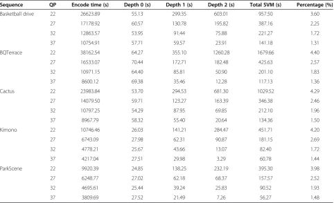
4.2. Additional overhead of SVM classification

SVM classification imposes additional computational complexity on encoder. Some experiments are conducted to investigate the overhead. Table 6 presents the total time to predict class labels in column “Total SVM” and the total time to encode sequences with the proposed algo-rithm in column “Encode Time”. As it shown in column

“percentage”, the computational overheads are not critical especially in the low bitrate cases, less than 5%. It costs a little more time to predict the class labels of CU 16 × 16 as there are more 16 × 16 CUs.

5. Conclusion

In this article, a CU splitting early termination algorithm is proposed. The CU splitting optimization in HEVC is formulized as a binary classification problem and is solved by support vector classification. In order to main-tain the RD performance of CU splitting early termi-nation algorithm, RD loss due to misclassification is introduced as weighting factor of training samples in the offline training procedure, with which the training method pays special attention to CUs which are prone Table 5 Complexity and RD performance comparison in

TS2 (average of 4 QP points)

Class Sequence Random access Low delay

ΔT(%) BDBR (%) ΔT(%) BDBR (%)

A PeopleOnStreet 37.94 1.8 – –

Traffic 62.58 1.8 – –

B BasketBallDrive 51.32 1.2 43.72 1.8

BQTerrace 52.16 0.6 44.03 0.7

Cactus 51.71 1.3 42.29 1.8

Kimono 56.75 1.0 50.14 1.8

C BQMall 45.18 2.2 44.03 3.3

PartyScene 34.33 1.1 27.51 1.8

RaceHorses 33.32 1.6 39.82 1.7

D BasketBallPass 39.06 1.5 36.80 1.7

BlowingBubbles 45.96 1.0 38.96 1.6

BQSquare 42.70 0.7 40.32 1.0

RaceHorses 29.74 1.2 29.86 1.4

E FourPeople – – 44.82 2.6

KristenAndSara – – 47.97 1.8

Average 44.83 1.29 40.00 1.77

Table 6 Computational complexity overheads of SVM prediction

Sequence QP Encode time (s) Depth 0 (s) Depth 1 (s) Depth 2 (s) Total SVM (s) Percentage (%)

Basketball drive 22 26623.89 55.13 299.35 603.01 957.50 3.60

27 17178.92 60.57 130.78 195.82 387.16 2.25

32 12863.57 53.95 91.44 75.88 221.27 1.72

37 10754.91 57.71 59.57 23.91 141.18 1.31

BQTerrace 22 38162.54 64.27 355.10 1260.28 1679.66 4.40

27 16533.07 70.44 172.71 182.48 425.63 2.57

32 10971.15 64.40 85.81 50.90 201.10 1.83

37 8600.12 69.38 35.46 12.28 117.13 1.36

Cactus 22 23983.84 53.70 294.53 681.30 1029.52 4.29

27 14079.50 59.71 123.27 163.39 346.38 2.46

32 10797.25 54.29 87.95 69.85 212.10 1.96

37 8967.79 58.32 55.40 20.64 134.36 1.50

Kimono 22 10746.46 26.03 141.21 284.47 451.71 4.20

27 6743.09 27.98 62.31 90.87 181.15 2.69

32 4778.21 25.67 43.66 13.07 82.40 1.72

37 4217.04 27.51 29.98 3.29 60.78 1.44

ParkScene 22 9920.39 24.85 138.25 232.19 395.30 3.98

27 6248.77 27.02 62.18 68.37 157.57 2.52

32 4695.61 25.44 39.24 25.83 90.52 1.93

to degrade RD performance when using a suboptimal partition. Furthermore, diverse features are considered such as the correlation between CUs both in spatial and temporal domains, prediction errors, motion activities, and RD cost of modes. To select the optimal feature subset, a wrapper feature selection approach is carried out. It embeds the model training into the selection process and simple greedy search is performed based on

F-score ranking. In such a way, the proposed algorithm performs well and stably across different configurations and various video contents. Since the CU splitting early termination model is trained offline and the optimal fea-ture subset is small, the proposed algorithm is computa-tionally simple. Demonstrated by the experimental results, the proposed algorithm can achieve 44.7% reduction in computational complexity with 1.35% BD-Rate increase in

“Random Access, main” configuration and 41.9% com-plexity reduction with 1.66% BD-Rate increase in “Low Delay, main”configuration.

Competing interests

The authors declare that they have on competing interests.

Acknowledgements

This work is supported by the National Basic Research Program of China (973) under Grant No. 2009CB320903 and Specialized Research Fund for the Doctoral Program of Higher Education (SRFDP) No. 20120101110032.

Received: 14 May 2012 Accepted: 20 December 2012 Published: 9 January 2013

References

1. ITU-T SG16 Q6 and ISO/IEC JTC1/SC29/WG11, 2010 ITU-T SG16 Q6 document VCEG-AM91 and ISO/IEC JTC1/SC29/WG11 document N11113,

Joint Call for Proposals on Video Compression Technology(ITU-T SG16 Q6 and ISO/IEC JTC1/SC29/WG11, Kyoto, Japan, )

2. L Bin, GJ Sullivan, X Jizheng,Comparison of compression performance of HEVC working draft 5 with AVC high profile(ITU-T/ISO/IEC Joint Collaborative Team on Video Coding (JCT-VC) document JCTVC-H0360, in 8th Meeting of JCT-VC, San Jose, USA, 2012)

3. B Bross, W-J Han, GJ Sullivan, J-R Ohm, T Wiegand,High efficiency video coding (HEVC) text specification draft 6(ITU-T/ISO/IEC Joint Collaborative Team on Video Coding (JCT-VC) document JCTVC-H1003, in 8th Meeting of JCT-VC, San Jose,USA, 2012)

4. J Kim, M Kim, H-Y Kim, K Sato, X Shen, L Yu, K Choi, ES Jang, B Bross, W-J Han, J-K Jo, S-N Park, DG Sim, S-J Oh,JCTVC TE9: Report on large block structure testing(ITU-T/ISO/IEC Joint Collaborative Team on Video Coding (JCT-VC) document JCTVC-C067, in 3rd Meeting of JCT-VC, Guangzhou, China, 2010)

5. Qualcomm Inc,Video Coding Using Extended Block Sizes, ITU-T Q.6/SG16 document COM16-C123-E(VCEG 36th Meeting, Geneva, Switzerland, 2009) 6. Z Liang, Z Li, M Siwei, Z Debin,Fast mode decision algorithm for intra

prediction in HEVC(2011 IEEE Visual Communications and Image Processing (VCIP), Tainan, 2011), pp. 1–4

7. T Su-Wei, H Hsueh-Ming, C Yi-Fu,Fast mode decision algorithm for residual quad-tree coding in HEVC(2011 IEEE Visual Communications and Image Processing (VCIP), Tainan, 2011), pp. 1–4

8. L Jie, S Lei, T Ikenaga, S Sakaida,Content based hierarchical fast coding unit decision algorithm for HEVC, 1st edn. (2011 International Conference on Multimedia and Signal Processing (CMSP), Guilin, Guangxi, 2011), pp. 56–59 9. K Jongho, J Seyoon, C Sukhee, C Jin Soo,Adaptive coding unit early

termination algorithm for HEVC(2012 IEEE International Conference on Consumer Electronics (ICCE), Las Vegas, NV, 2012), pp. 261–262

10. G Correa, P Assuncao, L Agostini, LA da Silva Cruz, Complexity control of high efficiency video encoders for power-constrained devices. IEEE Trans Consum Electron57(4), 1866–1874 (2011). doi:10.1109/TCE.2011.6131165 11. YM Lee, YJ Tsai, Y Lin, Improved motion estimation using early zero-block

detection. EURASIP J Image Video Process2008, 524793 (2008). doi:10.1155/2008/524793

12. K Byung-Gyu, Novel inter-mode decision algorithm based on macroblock (MB) tracking for the P-slice in H.264/AVC video coding. IEEE Trans Circuits Syst Video Technol18(2), 273–279 (2008). doi:10.1109/TCSVT.2008.918121 13. K Tien-Ying, C Chen-Hung, Fast variable block size motion estimation for H.264 using likelihood and correlation of motion field. IEEE Trans Circuits Syst Video Technol16(10), 1185–1195 (2006).

doi:10.1109/TCSVT.2006.883512

14. L Zhi, S Liquan, Z Zhaoyang, An efficient inter mode decision algorithm based on motion homogeneity for H.264/AVC. IEEE Trans Circuits Syst Video Technol19(1), 128–132 (2009). doi:10.1109/TCSVT.2008.2005804

15. ACW Yu, GR Martin, P Heechan, Fast inter-mode selection in the H.264/AVC standard using a hierarchical decision process. IEEE Trans Circuits Syst Video Technol18(2), 186–195 (2008). doi:10.1109/TCSVT.2007.913970

16. Z Huanqiang, C Canhui, M Kai-Kuang, Fast mode decision for H.264/AVC based on macroblock motion activity. IEEE Trans Circuits Syst Video Technol 19(4), 491–499 (2009). doi:10.1109/TCSVT.2009.2014014

17. Z Tiesong, W Hanli, S Kwong, C-CJ Kuo, Fast mode decision based on mode adaptation. IEEE Trans Circuits Syst Video Technol20(5), 697–705 (2010). doi:10.1109/TCSVT.2010.2045812

18. K Changsung, C-CJ Kuo, Feature-based intra-/inter coding mode selection for H.264/AVC. IEEE Trans Circuits Syst Video Technol17(4), 441–453 (2007). doi:10.1109/TCSVT.2006.888829

19. D Martinez-Enriquez, A Jimenez-Moreno, F Diaz-de-Maria, An adaptive algorithm for fast inter mode decision in the H.264/AVC video coding standard. IEEE Trans Consum Electron56(2), 826–834 (2010). doi:10.1109/TCE.2010.5506008

20. C Jui-Chiu, C Wei-Chih, L Lien-Ming, H Kuo-Feng, L Wen-Nung, A fast H.264/ AVC-based stereo video encoding algorithm based on hierarchical two-stage neural classification. IEEE J Sel Topics Signal Process5(2), 309–320 (2011). doi:10.1109/JSTSP.2010.2066956

21. C Chen-Kuo, P Wei-Hau, H Chiuan, Z Shin-Shan, L Shang-Hong, Fast H.264 encoding based on statistical learning. IEEE Trans Circuits Syst Video Technol21(9), 1304–1315 (2011). doi:10.1109/TCSVT.2011.2147250 22. K Jaeil, K Munchurl, H Sangjin, C In-joon, P Changsub,Block-mode

classification using SVMs for early termination of block mode decision in H.264| MPEG-4 part 10 AVC(Seventh International Conference on Advances in Pattern Recognition, ICAPR'09, Kolkata, 2009), pp. 83–86

23. C Corinna, V Vapnik, Support-vector networks. Mach Learn20(3), 273–297 (1995). 1995

24. B Scholkopf, C Burges, A Smola,Advances in Kernel Methods: Support Vector Learning(MIT Press, Cambridge, MA, 1999)

25. CW Hsu, CC Chang, CJ Lin,A practical guide to support vector classification, Tech. rep(Department of Computer Science, National Taiwan University, 2003). http://www.csie.ntu.edu.tw/cjlin/guide/guide.pdf

26. G Isabelle, E André, An introduction to variable and feature selection. J Mach Learn Res3, 1157–1182 (2003)

27. YW Chen, CJ Lin,Combining SVMs with Various Feature Selection Strategies

(Springer, New York, 2006)

28. HM Software. https://hevc.hhi.fraunhofer.de/svn/svn_HEVCSoftware/tags/HM-6.0. 29. F Bossen,Common test conditions and software reference configurations,

ITU-T/ISO/IEC Joint Collaborative Team on Video Coding (JCT-VC) document JCTVC-H1100(8th meeting o JCT-VC, San Jose, USA, 2012)

30. C Chih-Chung, L Chih-Jen, LIBSVM: a library for support vector machines. ACM Trans Intell Syst Technol2(27), 1–27 (2011)

31. G Bjontegaard,Improvements of the BD-PSNR model, ITU-T SG16/Q6 document VCEG-AI11(35th VCEG Meeting, Germany, Berlin, 2008)

doi:10.1186/1687-5281-2013-4