Continuation Methods for Nonlinear Flutter

Continuation Methods for Nonlinear Flutter

Edward E. Meyer

Boreal Racing Shells, Seattle, WA 98119, USA; [email protected]

Abstract: Continuation methods are presented that are capable of treating frequency-domain flutter equations including multiple nonlinearities represented by describing functions. A small problem demonstrates how a series of continuation processes can find all limit-cycle oscillations within a specified region with a reasonable degree of confidence. Curves of the limit-cycle amplitude variation with velocity, indicating regions of stability and instability with colors give a compact view of the nonlinear behavior throughout the flight regime. A continuation technique for reducing limit-cycle amplitudes by adjusting various system parameters is presented. These processes are economical enough to be a routine part of aircraft design and certification.

Keywords:aeroelasticity; multiple nonlinearity flutter; continuation methods; describing functions; bifurcation; continuation optimization; controlling LCO amplitudes

1. Introduction

In the commercial airplane industry certification that an aircraft is free from flutter instabilities is a major aspect of design and modification, requiring numerous analyses to cover the entire range of flight conditions and design parameters. Because it is impossible to analyze all flight conditions such as altitude, speed, fuel loading and payload, limited sets of conditions are analyzed, often relying on engineering judgment to pick the important conditions. To do the many analyses required, techniques are typically limited to linear, frequency-domain methods, using finite-element models reduced with low-frequency free-vibration modes, and linear unsteady aerodynamics from the doublet-lattice method.

Linear flutter equations assume infinitesimally small displacements; nonlinear flutter equations are far more realistic, allowing for limit-cycle oscillations (LCO), self-excited, constant amplitude oscillations that may be harmful or merely ride-quality problems depending on the amplitude. The additional information provided by nonlinear analyses is important to the design of commercial aircraft and should become a routine part of industrial flutter analyses.

Continuation methods, a class of methods for solving parameterized nonlinear equations [1], when applied to linear flutter equations have proven advantageous for covering the range of flight conditions by allowing for continuous variations in parameters, thereby reducing the number of discrete conditions necessary [2]. For example, interpolating mass matrices at several fuel loadings allows tracing the variation of flutter points with fuel loading in a continuous fashion. The success of continuation methods in treating linear flutter equations is due to the fact that in spite of the term linear flutter, the equations are nonlinear in a number of parameters, but linear in the generalized coordinates. Thus it is a small step to extend continuation methods to treat nonlinear flutter equations, identifying LCOs and tracing the variation of amplitude with parameters such as velocity.

modifications. The result is a method that is straightforward, efficient, and familiar to flutter engineers.

Following a brief summary of the continuation method presented in [2] and it’s application to nonlinear flutter equations, a small problem is used to illustrate the search for limit cycle oscillations. With a series of continuation processes the region of interest is covered with a grid of curves that find almost all LCOs in the region. Because of the sparsity of the grid an LCO is missed but is discovered using a continuation method that traces an optimal path toward a limit cycle. Starting from the limit cycles encountered, curves of LCO amplitude versus velocity are traced with continuation. From one of these curves at a specified velocity the optimal-path continuation method is used to reduce the LCO amplitude by adjusting gains and phases in a simple control system.

2. Continuation method

Continuation methods solve systems of nonlinear equations that are functions of more variables than equations, at discrete points over a range of the variables while maintaining continuity in the nonlinear functions. Continuity in flutter equations is important because there are always multiple solutions, known asaeroelastic modeswhich occasionally become close and difficult to distinguish.

The problem to solve is

f(x) =0∈Rm, x∈Rn, n>m (1)

starting from a known solutionx0and varying the independent variables through the desired range. n−mis the dimensionality of the solution: curves (1), surfaces (2), volumes (3), etc. The focus here is on curves:n=m+1.

The continuation method chosen to solve this is known as a pseudo-arclength method [1] with a minimum-norm corrector. At stepjthe next point is predicted using the tangent to the curve and the known solutionxj

x0_j+1=xj+αtj (2)

where the stepsizeαis an approximate distance along the curve, hence the name pseudo-arclength. Starting with the predictionx0_j+1the corrector iterates to find the solutionxj+1using a Newton-like method, computing correctionshisatisfying

J(xi)hi =−f(xi) (3)

and setting

xi+1=xi+hi, (4)

where

J(x) = f0(x) =

"

∂fi ∂xj

#

∈_Rm×n ₍₅₎

is the Jacobian matrix of derivatives of f with respect tox. The tangent vector (t) is characterized by

Jt=0, ktk2=

p

tTt=1, t= ∂x

∂τ (6)

whereτis the arclength along the curve.

Equation3is an underdetermined linear system that has an infinity of solutions; the smallest such solution can be computed using a QR factorization of the transposed Jacobian, splitting it into an(n,n)orthogonal matrixQtimes an(n,m)upper-triangular matrixR:

JT =QR= [Q₁ Q₂]

"

R1 0

#

Substituting Equation7into Equation3yields the minimum-norm solution ([7] pg. 300)

hi=−Q₁R−₁Tf(xi) (8)

Corrector iterations continue using Equations 3-8 until suitable convergence criteria are met, for example for some absolute toleranceeaand relative toleranceer:

kf(xi+1)k2<ea and khik2<ea+erkxi+1k2 (9)

In preparation for the next predictor step the tangent is computed from the (n,n−m)matrixQ2 in Equation7, a by-product of the QR factorization. Q₂is an orthogonal matrix spanning thenull spaceof the Jacobian,

JQ₂ = 0 ∈Rm×n−m

Q₂TQ₂ = I ∈_Rn−m×n−m ₍₁₀₎

An arbitrary vectorwis projected onto the null space with

¯

t=Q₂Q₂Tw=Q

"

0 0

0 I2

#

QTw ∈_Rn ₍₁₁₎

whereI2is the(n−m,n−m)identity andt=¯t/kt¯k2to satisfy Equation6. Ifn=m+1,Q2consists of one column, the projection only determines the sign of the tangent, and a logical choice for the vector to project is the tangent at the previous continuation step to keep the curve tracking in the right direction. In this case it is not absolutely necessary to do the projection, but it avoids forming

Q₂(see Section8) and is necessary for the optimal-path technique (Sections5.6,5.8and6).

3. Flutter Equations

Treating the flutter equation in the frequency domain has computational advantages over the time domain: the characteristic equation is a system of nonlinear algebraic equations instead of a system of differential equations which must be integrated at each flight condition. By contrast, the algebraic equations can be solved over a continuous range of flight conditions. The disadvantage is that nonlinearities must be approximated to conform to the harmonic motion assumption, Equation 12.

3.1. Assumed motion

Linear, frequency domain flutter analyses are based on the assumption that the actual motion of the structure (z) as a function of time is related to a set of complex generalized coordinates ( ˆq) by

z(t) =Φ<(qˆest) (12)

whereΦis typically a matrix of vibration modes,s=σ+iωis the Laplace variable,ωis the frequency, and oscillations are growing, neutral, or decaying if thegrowth factorσis positive, zero, or negative, respectively.

3.2. Equations

Various formulations of the flutter equations have been proposed [9–13]; any of them can be used with the continuation method presented above. A general form of the frequency-domain flutter characteristic equations is

h

s2M+sG+sV+ (1+id)K−qA(p,M) +Tiqˆ =Dˆqˆ =0, (13) whereM,K,G,V, A, andT are the (ns,ns) mass, stiffness, gyroscopic, viscous damping, unsteady aerodynamic, and control-system matrices, respectively,dis the structural damping coefficient,q = ρV2/2 is the dynamic pressure, p = s/V is the complex reduced frequency, V is the free-stream velocity, M = V/ais the free-stream Mach number, ais the sonic velocity, and ˆD is the complex dynamic matrix.

The related equation

ˆ

D(s)yˆ=0, kyˆk2=

q

ˆ

y∗yˆ=1, =(yˆk) =0 (14)

is a nonlinear eigenvalue problem withns solution eigenpair(si,yi), i = 1, . . .ns, normalized with the 2-norm ofyˆ1.0 and thekthcomponent real. Contrast this with the generalized-coordinate vector

ˆ

qwhich is a factor,ηtimesyˆ

ˆ

q=ηyˆ, kqˆk2=η (15)

This distinction is important when the dynamic matrix is a function of generalized-coordinate amplitudes, particularly whenηis small or zero.

3.3. Conversion to real

The continuation method presented is for real equations and variables; the flutter equations are converted from a set ofnscomplex equations to 2nsreal equations by setting

D=

"

<(Dˆij) −=(Dˆij) =(Dˆij) <(Dˆij)

#

y=

(

<(yˆi) =(yˆi)

)

q=ηy, (16)

so that

Dy=Dq=0 ∈_R2ns ₍₁₇₎

and the 2-norms of the eigenvectors and generalized-coordinate vectors are unchanged:

kyˆk2 =

q

ˆ

y∗yˆ=kyk2=

q

yT_y=1

kqˆk2 =

q

ˆ

q∗qˆ =kqk2=

q

qT_{q=η (18)}

where ˆ( )∗is the conjugate transpose.

3.4. Matrix parameterizations

Nonlinear structural elements such as freeplay and nonlinear stiffness can be approximated using describing functions, which conform to the harmonic motion assumption, Equation12. These stiffness elements are usually modeled with a single degree-of-freedom with no stiffness coupling between it and other degrees-of-freedom [4]. A describing function for bilinear stiffnesskjjassociated with generalized coordinatej, with stiffnessk0when the displacement amplitude|qˆj|is belowδand k1when it is above is

kjj(γ,r) = c(γ,r)k0

c(γ,r) =

  

r+_π2(1−r)hsin−1(γ) +γp1−γ2

i

ifγ≤1

1 otherwise

r = k1

k0, γ= δ |qˆj|

(19)

Nonlinear controls equations can be treated by describing functions [8]; one of the first multiple-nonlinearity flutter solutions was with structural nonlinearities in the control system [6].

3.5. Normalization

To make solutions unique a phase normalization on the generalized coordinates is necessary, for example by constraining thekth_{component of ˆqto be real:}

f_2ns+1==(qˆk) =q2k =0 (20)

If in additionηis to be held to a constant valueη0, another equation is added

f_2ns+2=qTq−η2₀=0 (21)

Therefore, to trace curves 2ns+2 independent variables must be used ifηis allowed to vary, or 2ns+3 if it is held constant.

3.6. Continuation formulations

The independent variables (x) comprise the 2ns variables y or q, plus enough additional parameters to give an underdetermined system. There are two cases to consider: constantη with 2ns+3 variables, and variableηwith 2ns+2 variables.

In what follows various combinations of velocity, frequency,σ, andηare used to demonstrate the solution technique; other parameters are possible but these three serve to illustrate typical analyses. Each combination of parameters will be named according to which three of these parameters vary; the fourth is implicitly constant. For example aV-σ-ωanalysis traces the variation inσandωwith velocity, holdingηconstant, as in a traditional linear flutter analysis, and aV-ω-ηanalysis traces LCO boundaries, the goal of this study.

3.6.1. Constantη

Solving the flutter equations with the generalized-coordinate norm held to a constant valueη0 presents a problem whenη0 = 0, and possibly numerical difficulties when η0 is small. The vector

For the demonstration parameters the equations are

f(x) =

     Dy

y2k

yTy−1

    

∈Rm

x =          V σ ω y         

∈Rm+1

q = η0y

J =

  

∂D ∂Vy

∂D ∂σy

∂D ∂ωy η0

∂D ∂qy+D

0 0 0 I2k:

0 0 0 2yT

   ∈R

m×m+1 ₍₂₂₎

whereI2k:is row 2kof the order 2nsidentity matrix.

3.6.2. Variableη

Ifηis allowed to vary the additional normalization Equation 21is not used so there arem = 2ns+1 equations: Equation17plus the phase normalization (Equation20),

f(x) =

(

Dq

q2k

)

∈_Rm ₍₂₃₎

and two of the three parameters (V,σ,ω) are needed.

Two combinations of the three parameters will be of interest,σ-ω-ηat constant velocity (used to search forσ=0) with

x=      σ ω q     

∈Rm+1 J=

" ∂D ∂σq ∂D ∂ωq ∂D ∂qq+D

0 0 I2k:

#

∈Rm×m+1 (23a)

andV-ω-ηat constantσ(used to trace LCO boundaries):

x=      V ω q     

∈_Rm+1 _J=

"

∂D ∂Vq

∂D ∂ωq

∂D ∂qq+D

0 0 I2k:

#

∈_Rm×m+1 _(23b)

If the first step in either of these processes starts from a known solution atη=0 with

x0=

     σ0 ω0 0     

or x0=

     V0 ω0 0      (24)

a modification in the tangent calculation is necessary, because the Jacobian and it’s null space vectors are then

J=

"

0 0 D

0 0 I2k:

#

, Q2=

  

1 0 0 0 1 0

0 0 y

 

The third column ofQ₂gives the desired greatest increase inη, so the first predicted solution for the σ-ω-ηprocess is

x0₁=x0+αt0=

    

σ0

ω0 0

    

+α

    

0 0

y

    

=

    

σ0

ω0 αy

    

(26)

In addition, an equation should be added to prevent converging to the trivial solution (q=0),

f2ns+2=q T_q−

η0=0 (27)

whereη0is the 2-norm of the predictedq. For the first stepη0=α.

4. Demonstration problem

A small, well-known problem illustrates the use of these continuation processes. The model is example 9-1 in [14], implemented as example HA145b in MSC-NASTRAN [13], with a generalized-coordinate basis of ns = 10 free-vibration modes and doublet-lattice aerodynamics. Bilinear nonlinearities are applied to the first 4 diagonals of the (diagonal) stiffness matrix using the describing function of Equation19withδ = 0.05,r = 2 (hardening) for diagonals 1 and 2,r = 0.5 (softening) for diagonal 3, andr=0.3 (softening) for diagonal 4.

5. Searching for limit cycle oscillations

Limit cycle oscillation is a condition where the structure is oscillating with an amplitude that is neither growing nor decaying; it is in dynamic equilibrium andσ= 0. On the other handq=0is a static equilibrium with stability determined by the sign ofσ. The goal then is to find all points within the region of interest whereσ=0.

The strategy is to find a number of points whereσ =0 using the formulations of Sections3.6.1 and3.6.2, then use these points to startV-ω-ηprocesses to trace the variation of LCO amplitude with velocity.

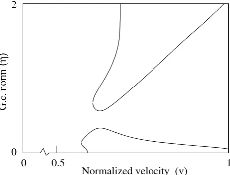
An example of the results of an LCO analysis is shown in Figure1 whereηis plotted against velocity normalized with respect to the maximum velocity of interest,v = V/Vmax. Ordinarily η would not be the plot variable of choice; instead, one or more of the nonlinear generalized-coordinate amplitudes would be plotted against velocity, but this choice is problem-dependent, soηis used for generality. Of the two curves in Figure1only the bottom one extends toη =0, so it is the only one which would be detected in a linear flutter analysis. Detecting the upper curve is why the processes of Sections3.6.1and3.6.2are necessary.

2

0

0.5 1

(η)

G.c. norm

0

Normalized velocity (v)

A systematic method for this search is to cover the range with a grid of V-σ-ωand σ-ω-ηprocesses, any of which might encounter σ = 0 points. Figure 2 shows a minimal grid of 6 lines where horizontal lines are V-σ-ωprocesses (numbered 1, 3, and 4) and vertical lines are σ-ω-ηprocesses (numbered 2, 5, and 6). Arrows indicate the direction of the continuation processes. Each of these lines represent one or more modes chosen to cover the frequency range of interest.

4

3

1

2 5 6

0

(η)

G.c. norm

Normalized velocity (v)

Figure 2.Grid for finding limit cycles

This set of processes is started from a free-vibration solution, at the origin of Figure2 (point 0), with v = η = 0. Two processes are started from this free-vibration solution: process 1, a V-σ-ωprocess along thevaxis and process 2, aσ-ω-ηprocess along theηaxis. The remaining vertical and horizontal grid lines are started from these two by interpolating to the desired points.

5.1. Point 0: free-vibration

AtV =0 the aerodynamic term drops out, and withη=0,qis zero for purposes of evaluating the dynamic matrixD. The problem to be solved then is in general the complex nonlinear eigenvalue problem, Equation14. Under certain conditions Equation 14 reduces to a polynomial eigenvalue problem [15], or to a generalized eigenvalue problem [16]. For example in the absence of controls equations, viscous and structural damping and gyroscopics the eigenvalue problem reduces to the real, generalized eigenvalue problem

h

−ω2M+K

i

z=0, y=

(

zi 0

)

(28)

Otherwise it is usually necessary to resort to nonlinear eigenvalue solution techniques [15].

Using the results of this eigensolution, representing the origin in Figure1, the LCO search is begun with two continuation processes corresponding to the two axes of Figure1: aV-σ-ωanalysis atη=0 (the horizontal orVaxis), and aσ-ω-ηanalysis atV=0 (the vertical orηaxis).

5.2. Process 1: V-σ-ω withη0=0

From these curvesσ-ω-η processes 5 and 6 on Figure2are started at the desired velocities by interpolating among solution points. Additionally, aV-ω-ηprocesses could be started from the point where a curve crosses theσ=0 axis, tracing the bottom curve in Figure1.

1

0

−1.5

0 1

Growth

Normalized velocity (v)

(σ)

Figure 3.Process 1:V-σ-ω analysis withη0=0

5.3. Process 2:σ-ω-η at V=0

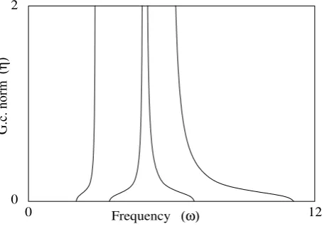
In aσ-ω-η processηis allowed to vary, velocity is held constant, and the equations are23and 23a. WithV=0 this process corresponds to the vertical axis of Figure1. Start points for this process are again select eigenvalues and eigenvectors from the free-vibration solution. At zero velocity the aerodynamic term drops out, so without viscous or structural dampingσ=0 and only the frequency changes with increasingη, as shown in Figure4.

Frequency 12

G.c. norm

0 0 2

(ω)

(η)

Figure 4.Process 2:σ-ω-η analysis withV=0

5.4. Processes 3 and 4: V-σ-ω

1.0

0.5

(σ)

0 12

−1 1

Growth

Frequency

(ω)

Velocity (v) η = 0

0

0 1

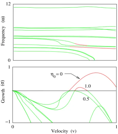
Figure 5.Processes 1, 3, and 4:V-σ-ωat 3 g.c. norms

5.5. Processes 5 and 6:σ-ω-η

σ-ω-ηprocesses 5 and 6 are started by interpolating the curves for each mode traced in process 1 to the desired velocity. Figure6showsσversusη at three velocities; for clarity only one of the 4 modes traced in process 1 is shown, the only one that encounters LCO.

G.c. norm

2

0

−1 0.5 2.5 5

v = 0 0.7

v = 0 0.5

0.7

0.5

Growth factor (σ) Frequency (ω)

(η)

Figure 6.Processes 2, 5, and 6:σ-ω-ηat 3 normalized velocities

5.6. Stability of equilibria

negative indicates stability. This derivative can be computed from the components of the tangent vector corresponding toσandq, recalling Equation6,

∂σ

∂η = ∂σ

∂τ ∂τ

∂η = tσ tη

, tη= ∂η ∂τ =

1 η

2ns

∑

qi∂qi ∂τ =

1 η

2ns

∑

qitqi (29)

whereτagain is the arclength along the curve. These tangent components are available at every step of aσ-ω-ηprocess, but this information is only relevant atσ = 0. More important is the stability of each point of LCO boundaries, created withV-ω-ηprocesses and Equation23b. That Jacobian then must be converted to the Jacobian of Equation23aby replacing the first column with∂f/∂σ,

¯

J= J+vut (30)

where

u=

    

1 0 .. .

    

∈_Rn v=

∂f

∂σ

−J:1 ∈Rm (31)

It is not necessary to actually make this replacement and re-factorize the Jacobian; only the vectors

u and v are of interest because with them the QR factorization of the transposed Jacobian can be updated ([7] pg. 334):

¯

JT= JT+uvt=QR+uvt=Q¯R¯ = _¯

Q1 Q¯2

"

¯ R1

0

#

(32)

Updating the factorization requires a small fraction of the work required to factorize the Jacobian. From the updated Jacobian the tangent used in Equation29is computed by projectingu onto the updated null space with Equation11:

t=Q¯2Q¯2Tu=Q¯

"

0 0

0 I2

#

¯

QTu ∈Rn (33)

Asηincreases or decreases from an unstable equilibrium the next equilibrium may be stable or unstable. Often an unstable equilibrium will be followed by a stable one; Figure6shows why this is true when the equilibriums are associated with the same aeroelastic mode. That this is not always true will be shown in Section5.8, where an LCO is discovered associated with a different aeroelastic mode.

5.7. Limit cycles: V-ω-ηanalysis atσ=0

2

0 1

0.5

Normalized velocity (v) 1

4

5 3

2

0.5 0.7 1

G.c. norm

(η)

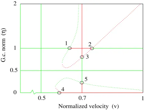
Figure 7.Start points for LCO curves

These points can be used to start V-ω-ηprocesses, the goal in this exercise, shown as dotted curves in Figure7. The upper dotted curve could be started from point 1, 2 or 3; either start point will trace the same curve. Likewise, the lower dotted curve could be started from point 4 or 5.

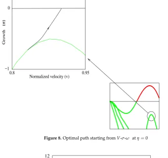
5.8. Optimal path: V-σ-ω-ηanalysis

Two of the grid lines in Figure2do not cross theσ = 0 axis (η = 0.5 in Figure5andv = 0.5 in Figure6) but come close. If all 4 parameters were allowed to vary instead of holding 1 fixed and varying the other 3 those 2 continuation processes might have also found limit cycle points. A continuation process where the number of unknowns is greater than the number of equations plus one requires only a minor modification of the continuation process, and is in a sense an optimization procedure.

The idea is to allow any number of independent variables greater than the number of equations (m) and to trace a special curve on the surface (or volume or higher-dimension manifold): the shortest path toward some goal, for example maximizing or minimizing some parameterβ. The key to tracing this curve is the tangent to the curve, computed by projecting the vector

w= ∂β ∂xi (34)

onto the null space of the Jacobian (Equation11). Aside from this modification, the continuation process is unchanged.

Here the goal isσ=0, a limit-cycle oscillation, and the equations are

f(x) =

(

Dq

q2k

)

∈R2ns+1 x=

         V σ ω q         

∈R2ns+3 (35)

Assuming the start point is at a negativeσ, the tangent vector is computed by projecting

w= ∂σ ∂xi =          0 1 0 0          (36)

Figures8and9show the result of such a process, starting at a mode in Figure3that peaks around v=0.9 andσ=−0.7, and continuing untilσ=0 is encountered.

0.95 Normalized velocity (v)

0.8 0

−1

Growth

(σ)

Figure 8.Optimal path starting fromV-σ-ω atη=0

12

11

−3 _{Growth (σ)} 0

(ω)

Frequency

Figure 9.Optimal path:σ-ω

1 0.6

Normalized velocity (v) 0.8

0

G.c. norm

(η)

Figure 10.LCO from optimal path

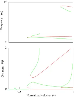
The complete set of LCO curves, with stable and unstable LCO again shown in green and red, is shown in Figure11.

2 12

(ω)

Frequency

2

0

Normalized velocity (v)

0.5 1

(η)

G.c. norm

Figure 11.Complete LCO boundaries

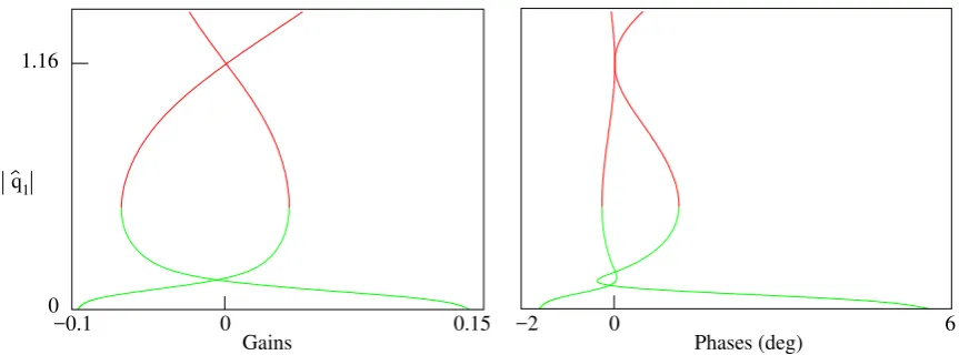
6. Decreasing LCO amplitudes

It is often desirable to reduce the amplitude of limit cycles, whether to avoid structural damage or to improve ride quality. Sometimes this can be done with structural changes such as reducing freeplay or increasing damping; in other situations such changes might be impractical and it may be necessary to resort to control systems. In either case the technique of Section5.8can be used to decrease the amplitude of a generalized coordinate undergoing LCO.

For example, including a simple control system (matrixT in Equation13) can be used to reduce the amplitude of generalized coordinate 1 in the unstable LCO at normalized velocity 0.8 in Figure 11. Details of the control system are unimportant, as it is just for illustration; it simply feeds back displacement in generalized coordinates 1 and 2 to add stiffness to these coordinates with 2 complex gains: g1eiφ1 _{and g2e}iφ2_{. The equation to be solved is as before, Equation23, withm= 2ns+2, but} now with three more unknowns than equations:

x=                  g1 φ1 g2 φ2 ω q                 

∈_R2ns+5 ₍₃₇₎

A projection vector pointing towards decreasing|qˆ1|is

w=−

∂|qˆ1| ∂xi =−                  0 0 0 0 0 wq                 

∈_R2ns+5 _w

q = q 1

q2 1+q22

           q1 q2 0 .. .            (38)

Beginning atv =0.8 on the upper curve in Figure11, whereη =1.18 and|qˆ1|=1.16, the projection vector guides the solution toward|q1ˆ | =0, as shown in Figure12. Stability of the LCO at each point on the curves is computed as in Section5.6.

Gains Phases (deg)

1.16

0

−0.1 0 0.15 −2 0 6

q₁

Figure 12.Reduction of an LCO amplitude with control system parameters

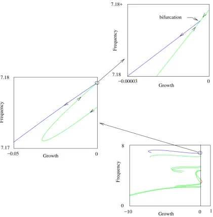
7. Bifurcation

a rank-deficient Jacobian matrix, and a change in the sign of the determinant of the Jacobian matrix augmented with the tangent vector. It can be shown [1] that a change in the sign of

µ(x) =det

"

J tT

#

=dethJT ti (39)

indicates a bifurcation has been passed. A method for computing µis shown in Section 8 that is economical enough that it could (and should) be done at every step.

One of the curves in theV-σ-ωprocess shown in Figure5encounters a bifurcation, although it is not evident at that scale. When plottedσversusωwith an expanded scale the bifurcation becomes more evident, as shown in Figure13. Arrows indicate the direction of positive determinant. Had the bifurcation not been detected the process would have tracked only the green curve. Detecting the bifurcation and computing the bifurcation tangent allows the blue curve to be traced.

Frequency

7.18+

7.18 −0.00003

Growth 0

bifurcation

7.18

7.17

−0.05 _Growth 0

Frequency

1 Growth

Frequency

8

0

−10 0

Figure 13.Bifurcation in aV-σ-ωprocess

Branching from the bifurcation requires the tangent to the branch curve. For a simple bifurcation atxb, detected by a change in the sign ofµ(x), the Jacobian will have 1 rank deficiency, and theQ2 matrix has 2 columns, some combination of which gives the branch tangent, and another combination continues the original curve.

A singular value decomposition (SVD) ([7] pg. 76) of the Jacobian atxb,

J=UΣVT, U∈_Rm×m_{, V ∈}

Rm+1×m+1 (40)

reveals the rank and is necessary for branching from the bifurcation. The last column ofU(um), and the last two columns ofVT(vmandvm+1) are left and right null vectors of the Jacobian, and the two tangents emanating from the bifurcation are combinations of these:

tk=αkvm+βkvm+1, k=1, 2. (41)

where

αk =

ck

q

c2_k+a2₁₁

= _q a22 c2_k+a2₂₂

,

βk =

ck

q

c2 k+a222

= _q a11 c2

k+a211 a11 = ∂

2_g ∂ξ2₁ ≈

1

e2[g(e, 0)−2g(0, 0) +g(−e, 0)] a12 =

∂2g ∂ξ1∂ξ2

≈ 1

4e2[g(e,e) +g(−e,−e)−g(e,−e)−g(−e,e] a22 =

∂2g ∂ξ2₂

≈ 1

e2[g(0,e)−2g(0, 0) +g(0,−e)] e ≈ 10−6

g(ξ1,ξ2) = uTmf(xb+ξ1vm+ξ2vm+1) (42) One of these tangents is aligned with the original curve, the other with the bifurcation curve. Comparing with the previous tangent (tj) determines which is the primary tangent (tc) and the bifurcation tangent (tb):

t1= t

T jt1

, t2= t

T jt2

tc,tb =

(

t1,t2 if t1>t2

t2,t1 otherwise

(43)

8. Programming considerations

Much of the computational effort in the continuation method is in the factorization of the Jacobian matrix in Equation7, where QR factorizations are used to solve the underdetermined system. Some continuation methods [1,18] add an equation in the corrector phase to constrain corrections, for example to hold one of the variables constant, creating a square set of linear equations that can be solved using an LU factorization instead of QR. Theoretically LU is faster than QR but QR is more stable and modern computer architectures eliminate the speed advantage ([7], pg. 299). QR is also necessary for the optimal-path technique of Section5.8.

The LAPACK library [16] provides several variants of QR factorizations; the preferred routine for efficiency and stability isSGEQP3([16] sect. 2.4.2.3). None of the QR routines in LAPACK return the

subroutineSTRSMsolves a set of equations with it. SubroutineSORMQRis provided to multiplyQ

orQTby a vector.

Projecting a vector onto the null space of the Jacobian can be done in LAPACK without actually forming theQ2matrix with two calls to subroutineSORMQR:

Q₂QT₂w=Q

"

0 0

0 I2

#

QTw (44)

that is, callSORMQRto multiply the vector byQTzero the firstmelements of the result, then call it again to multiply byQ.

Updating the QR factorization to determine stability with Equation32can be done efficiently with theqrupdatepackage available at [19].

Evaluating the determinant in Equation39 is simplified by recognizing that the tangent came from the QR factorization, that the determinant of an orthogonal matrix is±1, and the determinant of a triangular matrix is the product of the diagonals. Furthermore, the tangent and the QR factorization of the Jacobian it was computed from are available from the last corrector iteration, so the desired determinant is simply

dethJT ti = det[QR t] =det[Q₁ Q₂]

"

R 0

0 γ

#

= γdetQdetR= (−1)kγ m

∏

Rii (45)

wherekis the number of non-zero elements in theTAUarray [20] for LAPACK QR routines, andγis 1 if the last element ofQTwis positive or -1 if it is negative.

Derivatives are an essential part of continuation methods. Accurate derivatives of parameters and matrices with respect to the independent variables are necessary for computing the Jacobian matrix that is used both to iterate to solutions and predict the next solution. Deriving formulas for complicated expressions like Equation19can be tedious and error-prone. A technique that eliminates the need for closed expressions for the derivatives and can reduce coding errors is automatic differentiation [21]. This programming technique gives exact derivatives at a cost on the order of evaluating the function itself, in contrast with the other alternative, difference approximations, which are not exact and much more expensive to compute. The autodiff.org [22] website is devoted to automatic differentiation resources.

9. Conclusions

A continuation method capable of treating frequency-domain flutter equations with multiple nonlinearities approximated with describing functions has been developed. With it a set of continuation processes can find with reasonable certainty all limit-cycle oscillations within a desired flight envelope, tracing curves of limit-cycle amplitude versus velocity and indicating stability with colors.

With a small modification to the continuation method curves can be traced taking an optimal path with respect to any number of parameters toward some goal. This technique was used to seek out a limit cycle that was missed, and to reduce limit-cycle amplitudes by adjusting control-system parameters.

References

1. Allgower, E.L.; Georg, K. Numerical Continuation Methods: an Introduction; Vol. 13, Springer Series in Computational Mathematics: Berlin, 1990.

2. Meyer, E.E. Unified Approach to Flutter Equations. AIAA Journal2014,52, 627–633.

3. Shen, S.F. An Approximate Analysis of Nonlinear Flutter Problems. Journal of the Aerospace Sciences1959, 26, 25–32.

4. Gordon, J.T.; Meyer, E.E.; Minogue, R.L. Nonlinear Stability Analysis of Control Surface Flutter with Freeplay Effects.Journal of Aircraft2008,45, 1904–1916.

5. Lee, C.L. An Iterative Procedure for Nonlinear Flutter Analysis. AIAA Journal1986,24, 833–840.

6. Breitbach, E.J. Flutter Analysis of an Airplane with Multiple Structural Nonlinearities in the Control System. TP 1620, NASA, 1980.

7. Golub, G.H.; Van Loan, C.F. Matrix Computations, fourth ed.; The Johns Hopkins University Press: Baltimore, 2013.

8. Gelb, A.; Vander Velde, W.E. Multiple-Input Describing Functions and Nonlinear System Design; McGraw-Hill: New York, 1968.

9. Hassig, H.J. An Approximate True Damping Solution of the Flutter Equation by Determinant Iteration. Journal of Aircraft1971,8, 885–889.

10. Chen, P.C. Damping Perturbation Method for Flutter Solution: the g-Method. AIAA Journal2000, 38, 1519–1524.

11. van Zyl, L.H.; Maserumule, M.S. Divergence and the pk Flutter Equation. Journal of Aircraft 2001, 38, 584–586.

12. Edwards, J.W.; Wieseman, C.D. Flutter and Divergence Analysis Using the Generalized Aeroelastic Analysis Method. Journal of Aircraft2008,45, 906–915.

13. Rodden, W.P. MSC/NASTRAN Handbook for Aeroelastic Analysis; The MacNeal-Schwendler Corporation: Santa Ana, California, 2009; pp. 357–372.

14. Bisplinghoff, R.L.; Ashley, H.; Halfman, R.L.Aeroelasticity; Addison-Wesley: Reading, Mass., 1955. 15. Ruhe, A. Algorithms for the Nonlinear Eigenvalue Problem. SIAM Journal on Numerical Analysis1973,

10, 674–689.

16. Anderson, E.; Bai, Z.; Bischof, C.; Blackford, S.; Dongarra, J.; Du Croz, J.; Greenbaum, A.; Hammarling, S.; McKenney, A.; Sorensen, D.LAPACK Users’ Guide, 3rd ed.; Siam, 1999.

17. Meyer, E.E. Continuation and Bifurcation in Linear Flutter Equations. AIAA Journal2015,53, 3113–3116. 18. Rheinboldt, W.C.; Burkardt, J.V. A Locally Parameterized Continuation Process. ACM Transactions on

Mathematical Software (TOMS)1983,9, 215–235.

19. Hajek, J.https://sourceforge.net/projects/qrupdate/, 2009.

20. Langou, J.http://icl.cs.utk.edu/lapack-forum/viewtopic.php?f=2&t=1741, 2010.

21. Griewank, A.; Walther, A. Evaluating Derivatives: Principles and Techniques of Algorithmic Differentiation, second ed.; Siam, 2008.

22. http://www.autodiff.org.

c