Improving the Scalability of Wireless Sensor Networks
by Reducing Sink Node Isolation
Fagbohunmi Griffin Siji
Computer Science Department Abia State Polytechnic Aba
Abia State, Nigeria
Eneh I.I
Department of Electrical & Electronics Engineering, Enugu State University of
Science & Technology, Enugu State Nigeria
ABSTRACT
The aim of this paper is to investigate the rate in which sink node isolation occur in order to improve the scalability of wireless sensor networks. It can be noted that while most previous works investigate scalability in terms of total energy consumption or the rate of node’s death in the WSN. In this work, we consider the scalability in terms of the rate of sink node isolation with respect to the WSN deployment size. The aim of power-aware routing algorithms in Wireless Sensor Networks (WSNs) is to solve the key issue of prolonging the lifetime of resource-constrained ad-hoc sensor nodes. Contemporary WSN routing algorithm designs have severe limitations on their scalability; that is, large-scale deployments of WSNs result in relatively shorter lifetimes, as compared to small-scale deployments, primarily owing to rapid sink node isolation caused by the quick battery exhaustion of nodes that are close to the sink. This paper analyzes the scalability limitations of conventional routing algorithms and compares them to the recently proposed Improved MultI-layer routiNg (IMIN). IMIN will be mathematically analyzed to show the relationship between network size and routing algorithm scalability. Additionally, through extensive simulations, it will be deduced that IMIN scales considerably better in terms of network connectivity.
Keywords
Node isolation, Scalability, WSN deployment, hierarchical routing, cluster head, cluster member, Sink connectivity area
1.
INTRODUCTION
The advancement in wireless communications technology and nanotechnology have facilitated the deployment of Wireless Sensor Networks (WSNs), which consist of inexpensive sensor-equipped wireless-transmission capable nodes that are deployed in large numbers to monitor areas of interest. Applications where sensors are used include measuring temperature readings, to military, which include detecting adversary movements.
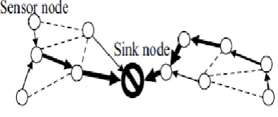
The structure of a WSN, as illustrated in Fig. 1, is made up of sensor nodes and a sink node. The sensor nodes collect data from their surroundings and forward them to the sink node. In ad-hoc networking there is a lack of infrastructure support, hence individual nodes acts as routers by performing the packet forwarding role. Additionally, since ad-hoc networking is used to compensate the lack of infrastructure. The sink node acts as the gateway for the WSN, an assembly point from which the user extracts data from the WSN. Sensor nodes in WSNs are battery-powered devices. Whenever the battery of a sensor node is used up, the node can no longer operate, this result in a partial loss of network functionality, replacement of a large number of batteries in some applications is impractical, and hence power-efficient technologies are
required to ensure long lifetimes of WSNs. Consequently, much research effort has been put into power-aware routing algorithms for WSNs, and the scalability of these algorithms has been evaluated from different perspectives. This paper focuses on routing algorithm designs that have good scalability for large-scale WSN deployments.
Figure 1: Flat multi-hop routing
A scalable WSN routing algorithm must work well as the network grows large. As the network size grows, the volume of data relayed to the sink node grows, and consequently the load on the network increases, especially on nodes that are close to the sink, since in most cases they represent the shortest route to the sink. Consequently the death rate of sensor nodes closer to the sink increases, thus leading to early sink node isolation. As a result, the lifetime of a large WSN deployment is shorter than that of a small WSN deployment. This problem can be easily overcome in the case where the sink node is mobile so as to avoid sink node isolation as in [1], [2]. In [3], multiple sinks are deployed to divide the network load in a more uniform manner. This work considers a 3-level hierarchical heterogeneous routing algorithm that scales well as the network grows larger. This is an improvement on the HYMN protocol where a 2- level hierarchical routing algorithm was proposed as in LEACH. The motivation for this came from the fact that with a 3-level hierarchical structure, nodes farther from the sink form another level of clusters with separate cluster heads. This effectively reduces the amount of data packet transfer in the SCA, which ultimately reduces significantly the sink-node isolation.
2.
RELATED WORKS
To prolong the longevity of a WSN, the energy consumed by the WSN per unit of data collected from the monitored area must be minimized. Many routing algorithm have been proposed trying to meet this objective. These can be widely classified as flat multi-hop routing algorithms and hierarchical
multi-hop routing algorithms. In the following two subsections, we examine these two categories.
2.1
Flat multi-hop Routing Algorithms
This category of algorithms aims to minimize the total power consumption used for sending data to the sink node.
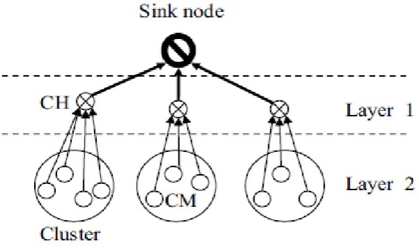
Figure 2: Hierarchical multi-hop routing
Fig. 1 illustrates how a flat multi-hop routing algorithm routes data. Each node can communicate with other nodes that are within its maximum transmission range, and an arrow’s width is proportional to the amount of data being transmitted between a pair of nodes. The utilization of a single communication link differs with different routing algorithms. For example, the algorithms proposed in [4], [5] are designed to minimize the total power consumption of the network. The cost of using a link is defined according to the following equations.
linkcost (i,j) = es(i) + er(j) (1) es(i) = Є1d2i,j + Є2 (2)
er(j) = Є3 (3) Here, the cost of sending data over from node i to node j, linkcost(i, j), is composed of two parts, cost on sender es(i) and the cost on the receiver er(j). The term es(i) is proportional to the square of distance di,j between node i and node j, while Є1 and Є2 are constants dependent on the sending node’s transmission circuit. The term er(j) is a constant Є3 dependent
on the receiving node’s receiving circuit. If the route where the sum of all link costs is minimum is used, the WSN’s total power consumption can be minimized, thereby effectively prolonging the lifetime of the network.
While the above algorithm minimizes the total power consumption of the WSN, it overburdens certain nodes, leading to their quick battery exhaustion. To solve this problem, linkcost function is redefined as follows,
linkcost (i,j)uniform = (4)
By dividing linkcost(i, j) by the residual energy of the Sending node , the probability of node being chosen decreases as its residual energy decreases. In [5], n is set to be 2, enabling a uniform distribution of power consumption over
all nodes and at the same time minimizing the total power consumption of the WSN.
2.2
Hierarchical Multi-hop Routing
Algorithms
While flat multi-hop routing algorithms successfully route data to minimize the power consumption of the WSN, they fail to take advantage of the nature of data collected by the WSN. The application area and the relatively high node density make the data collected by the WSN highly redundant, thus making data aggregation very attractive in WSNs. Hierarchical multi-hop routing algorithms take advantage of the highly-correlated nature of WSN’s collected data, and sensor nodes assume different roles. We describe the most notable example of hierarchical multi-hop routing algorithms, dubbed Low-Energy Adaptive Clustering Hierarchy (LEACH) [6], to illustrate their operation.
LEACH, as illustrated in Fig 2, is a two-leveled hierarchical routing algorithm in which nodes can take one of two different roles, a Cluster Head (CH) or a Cluster Member (CM), and these roles are changeable in a unit of time referred to as a Round. At the start of every Round, some nodes take the role of CH with a specific probability, and the rest of the nodes become CMs. Each CM chooses a single CH, and a Cluster is formed from a single CH and a few CM(s). Each CM sends its sensed data to its corresponding CH, and each CH aggregates its own sensed data and the data it collected from its CMs, and sends them to the sink node. CHs transmit directly to the sink node. They are small in number compared to the CMs, hence the amount of energy consumed tend to be high per single hop-sink transmission. This results in quick battery discharge (drainage) of the CHs.
and CMs can be decreased, thus resulting in reduction of power consumption in each cluster. On the other hand, in PEACH [8], by increasing the probability of the node with the highest remaining power to become a CH, fairness in power consumption can be improved. Since the number of nodes used to relay data is relatively small, the transmission distance tends to be large, thus resulting in low-efficiency transmissions. Nevertheless, hierarchical multi-hop routing algorithms are an excellent approach in terms of their ability of capitalizing on the highly correlated nature of data in WSN.
2.3
Scalability in WSNs
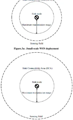
In this section, a taxonomy of WSN’s structure is presented, to classify the importance of specific nodes over other nodes in the WSN. In wireless multi-hop networks, nodes that lie within the interior of the maximum transmission range of the sink node are provisioned connectivity with the nodes outside its maximum transmission range, through multi-hop transmission, as illustrated in Fig. 3. We refer to this area as Sink Connectivity Area (SCA). As can be observed from Fig. 1, owing to the many-to-one (converge-cast) traffic patterns in the WSN, the amount of data relayed per node increases as the node’s position gets closer to the sink node, in effect, shortening its lifetime.
Figure.3a: .Small-scale WSN deployment
Figure 3b: Large-scale WSN deployment Figure 3: Sink Connectivity Area (SCA)
Generally, the nodes in the SCA have much shorter lifetimes than nodes outside the SCA; in the event that all the SCA nodes die, the sink node will not be able to collect data from the WSN, practically making the WSN non-functional; we refer to this problem as sink node isolation. As shown in Fig.
evaluate the scalability of a WSN routing algorithm, it is essential to take into account the rate in which sink node isolation occurs, while most previous works investigate scalability in terms of total energy consumption or the rate of node’s death in the WSN [8]. In this work, we consider the scalability in terms of the rate of sink node isolation with respect to the WSN deployment size. We present the recently proposed algorithm dubbed Improved MultI-hop routiNg (IMIN) and show its superior scalability as compared with contemporary WSN multi-hop routing algorithms.
LAYER 1
LAYER 2
LAYER 3
Cluster
CH
2CH
1Sink Node
Figure 3 A 3-layer Hierarchical Multi-hop Routing
3.
IMPROVED MULTI-HOP ROUTING
ALGORITHM
In general, the number of nodes in the SCA is much less than the nodes outside the SCA; inevitability, the volume of data they sense is insignificant as compared with the data they relay. Additionally, while the WSN’s size can grow, the SCA’s size is constant, implying that to increase the scalability of the WSN with respect to the rate of sink node isolation, the growth rate of flows needs to be limited as the WSN grows in size, and/or the cost of relaying data to the sink node needs to be minimized. The proposed algorithm IMIN achieves both solutions by using a 3-level hierarchical multi-hop routing algorithm to limit the inflow of data from outside the SCA, while using a third level Cluster head CH2 to limit the data inflow due to CH1 inside the SCA. This ultimately minimizes the transmission packets of nodes inside the SCA.
3.1
Routing Outside The SCA
Since transmission power consumption is proportional to the volume of data being relayed in the SCA, limiting the volume of data inflow into the SCA is essential. Applying a 3-level hierarchical multi-hop routing algorithm limits the volume of data inflow to the SCA, thus effectively reducing the load on the SCA. This method continues to be effective as the size of the WSN grows, by reducing the volume of data flow.
3.2
Routing inside the SCA
Inside the SCA, the most important objective of the applied routing algorithm is to minimize the amount of data packets
inside the SCA while relaying the data flowing in from outside the SCA. This objective can be successfully achieved by applying the 3-level hierarchical multi-hop routing.
3.3
Optimal location of Level 2/3 boundary
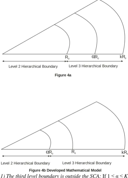
This section briefly discusses the required size of level 2 in order to optimize IMIN. This concept was addressed in [9] where the idea of multi-layer boundary was discussed. In this paper the multi-layer boundary is defined as the location where the employed routing is changed from level 2 to level 3, and vice versa. The analytical model is illustrated in Fig. 4, with its parameters listed in Table 1. The problem was divided into two cases, the case where the boundary is outside the SCA, and that inside the SCA.
Level 2 Hierarchical Boundary Level 3 Hierarchical Boundary
Level 2 Hierarchical Boundary Level 3 Hierarchical Boundary
α
R0 R0 kR0α
R0 kR0R0
Figure 4a
Figure 4b Developed Mathematical Model
1) The third level boundary is outside the SCA: If 1 ≤ α ≤ K, as shown in Fig. 4(a), power consumption in the SCA, EOUT, is attributed to two components, as follows:
EOUT = + (5)
where and denote the energy consumed to transfer the data that was sensed from inside the SCA to the sink node, and that for relaying data flowing into the SCA
from outside to the sink node, respectively. and are equal to:
= πmρ R0
3
(6)
= πmρ R
0 3
{k
2ϒ + (1- ϒ) α2
– 1} (7)
flowing into the SCA. It is worth noting that this result is independent of the WSN deployment size, KR0.
2) The third level boundary is inside the SCA: If 0 ≤ α ≤ 1 as shown in Fig. 4(b), EIN, the energy consumption in the SCA, is attributed to four components, as follows:
EIN = + + + (8)
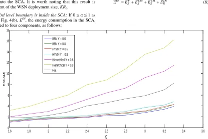
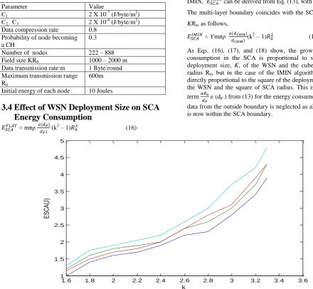
Figure 5a: Effect of WSN Deployment Growth on Energy Consumption in the SCA
where denotes the energy consumed to transfer the data that was sensed from inside the interior of αR0 to the sink node. is the energy consumed when CMs send data sensed from the SCA to their respective CHs, and is the energy consumed by CHs in the SCA when they send their aggregated data to the sink node. is the energy consumed for relaying data coming from outside the SCA to the sink node by both layer 2 and layer 3 CH nodes within the SCA. They are equal to:
= πmρ α3R03 (9)
= mρR02
(1 - α2)ρ (1 – δ) e(dCM) (10)
= πmρϒ R03
* { (α3– 3α + 2) +
3α(1 - α2) (11)
= πmρϒ R03 * {( α4– 4α2 + 2) +
3α(α3 – 3α + 2)
+ 5α(1-α
2
) } (12)
= m ϒ R
02 (k2 – 1) ρ * {
e(dCH2)
+
e (dF )} (13)
EIN can be rewritten in the following polynomial form, EIN = A1α4 + A2α3 + A3α2+ A4α + A5 (14)
Table 1.Problem Preliminaries
Parameter
dF Average distance between nodes in each level of the hierarchical structure dCH1 Average transmission distance for CH in
level 2 hierarchy
dCH2 Average transmission distance for CH in level 3 hierarchy
dCM Average distance between CH and CMs e(d) Power consumption over distance d
R0 SCA radius
Α Factor of third level boundary 0 ≤ α ≤ K k Factor of sensing field
ρ Node density
δ CH ratio 0 < δ < 0.5
m Message size
ϒ Data compression ratio 0 < ϒ ≤ 1
where the signs of the coefficients are A1>0, A2<0,A3<0, and A4<0. To understand the shape of this function by applying the first derivative test, we have
(EIN) = 4A1α3 + 3A2α2+ 2A3α + A
4 (15)
If α is 0, i.e., only 2-level hierarchical multi-hop routing is used, (EIN)= A4<0 which reflects that the function has a negative gradient; in other words, energy consumption decreases as the boundary between the 2nd and 3rd layer cluster heads move away from the sink, and from Eq. (7), we conclude that the optimal boundary location is inside the SCA. Computer simulations were conducted to locate the optimal boundary for nodes in level 2 and level 3. Further simulation was also carried out to measure how the energy consumption of the SCA changes with respect to the boundary. The simulation results confirmed the mathematical model. It is interesting to note that the optimal layer boundary
1.6 1.8 2 2.2 2.4 2.6 2.8 3 3.2 3.4 3.6
0 2 4 6 8 10 12 14 16 18
K
E
S
C
A
(
J
)
exists inside the SCA area, and it is intuitive that the optimal boundary overlaps with the SCA if the compression rate is equal to 1.0, i.e., no data compression.
On the other hand, as the compression rate and the CH ratio improve, setting the CHs boundary inside the SCA can further decrease the energy consumption of the SCA. The main contribution of the 3-level hierarchical routing algorithm is that unlike in HYMN the energy consumption of the SCA does not increase as the size of the WSN routing area increases beyond a specific degree due to increase in transmission packet inside the SCA. This is not the case with the IMIN algorithm as the number of data packets relayed by the layer 2 CHs has been minimized by the introduction of layer 3 CHs.
Table 2. Configuration of Simulation Environment
Parameter Value
Є1 2 X 10⁻⁷ (J/byte/m2)
Є2, Є3 2 X 10⁻⁶ (J/byte/m2) Data compression rate 0.8
Probability of node becoming a CH
0.3
Number of nodes 222 – 888 Field size KR0 1000 – 2000 m Data transmission rate m 1 Byte/round Maximum transmission range
R0
600m
Initial energy of each node 10 Joules
3.4
Effect of WSN Deployment Size on SCA
Energy Consumption
= mπρ(k2 – 1) (16)
The energy consumption attributed to KR0 in the case of hierarchical multi-hop routing algorithms, can
be derived from Eq. (13), with α = 0, as follows:
= ϒmπρ (k2 – 1) (17)
The energy consumption attributed to KR0 in the case of HYMN, can be derived from Eq. (13), with α = 1, where the optimal hybrid boundary coincides with the SCA for a large KR0, as follows,
= ϒmπρ (k2 – 1) (18)
The energy consumption attributed to KR0 in the case of IMIN, can be derived from Eq. (13), with α = 1, as The multi-layer boundary coincides with the SCA for a large KR0, as follows,
= ϒmπρ (k2 – 1) (19)
As Eqs. (16), (17), and (18) show, the growth of energy consumption in the SCA is proportional to square of the deployment size, K, of the WSN and the cube of the SCA radius R0, but in the case of the IMIN algorithm (19), it is directly proportional to the square of the deployment size K of the WSN and the square of SCA radius. This is because the term e (dF ) from (13) for the energy consumed in relaying data from the outside boundary is neglected as almost all data is now within the SCA boundary.
Figure 5b: Effect of WSN deployment size growth on energy consumption in the SCA with IMIN, and HYMN graph amplified
1.6 1.8 2 2.2 2.4 2.6 2.8 3 3.2 3.4 3.6
1 1.5 2 2.5 3 3.5 4 4.5 5
k
E
S
C
A
(J
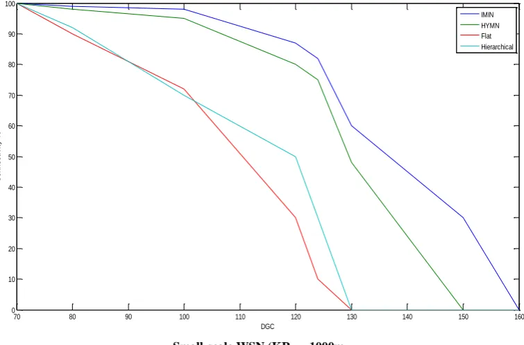
Small-scale WSN (KR0 = 1000m
Figure 6a: Scalability in terms of connectivity
(b) Large-scale WSN (KR0 = 2000m)
Figure 6b: Scalability in terms of connectivity
This is possible because the CHs for the third layer is made to be close to the sink. This however causes the probability of a node to become cluster head in IMIN to be higher. Additionally, the transmission distance in the SCA is an important factor. IMIN successfully utilizes the minimum transmission distance of 3- layer routing algorithms, dCH. On
the other hand, the HYMN routing algorithms suffer from longer transmission distance, dCH. Especially for nodes outside the SCA. Thus it is deduced from Eqs (15), (16), (17) and
(18) that IMIN has superior scalability. For illustrative purposes Eqs (15), (16), (17) and (18) is plotted as shown in Figure 5. dCH, dCHM and dF can be estimated from the node density and cluster head ratio by following the parameters listed in Table 2. It can also be noted that a node in IMIN has a higher probability of being a cluster head due to the higher rate of energy depletion experienced in layer 3. The parameter K is varied to correspond to a field size KR0 ranging from 1000m to 2000m
70 80 90 100 110 120 130 140 150 160
0 10 20 30 40 50 60 70 80 90 100
DGC
C
o
n
n
e
c
ti
v
it
y
%
IMIN HYMN Flat Hierarchical
10 20 30 40 50 60 70
0 10 20 30 40 50 60 70 80 90 100
DGC
C
o
n
n
e
c
ti
v
it
y
%
3.5
Experiment Setup
MATLAB version 2008 was used to execute the experiments. Sensor nodes are placed in a random uniform manner within a circular sensing field centered on the sink node. Table 2 shows the configuration of the simulation environment where the value of environmental parameters is set according to the configurations reported in the following references [6], [10]. Since the maximum transmission range of the nodes is 600m, the SCA is also a circular area with a radius of 600m having its center on the sink node. It was assumed that the nodes are distributed without large deviation in node density, i.e., the number of nodes in the SCA does not deviate much to accurately measure the scalability in the conducted experiments. The experiment is set so that all nodes in the WSN send a single packet in a period of time, referred to as Data Gathering Cycle (DGC), and all packets need to be routed to the sink node. To illustrate the concept of IMIN, Toh’s method and a multi-hop variant of LEACH have been employed inside and outside of the SCA, respectively. Also, three notable multi-hop routing algorithms, as respective representative flat, hierarchical and hybrid multi-hop routing algorithms have been used to compare with IMIN.
3.6
Scalability in Terms of Sink Node
Isolation Rate
The scalability of the three categories of WSN multi-hop routing algorithms was investigated with respect to sink node isolation rate, i.e., how long can the WSN sustain connectivity before network partition occurs with respect to WSN deployment size, KR0. As a metric, Connectivity was used as a measure of the number of DGCs before sink node isolation occurs. Connectivity can be defined as follows:
Connectivity = (20)
IMIN successfully sustains Connectivity for the longest period of DGCs as compared to flat, hierarchical multi-hop routing and HYMN algorithms. As evident from this result, we can conclude that IMIN decreases the rate of sink node isolation, thus improving the scalability of a WSN.
4.
CONCLUSION
This paper has investigated the scalability limitations in large wireless sensor network deployments. Wireless sensor network routing algorithms can be widely categorized into two categories, flat multi-hop routing algorithms which have an excellent ability in minimizing the total power consumption of the network by using small transmission distances, and hierarchical multi-hop routing algorithms which decrease the volume of data flowing in the network by taking advantage of the highly correlated nature of the collected data by applying data aggregation. It was shown that in both categories, large-scale deployments have experienced relatively shorter lifetimes as compared to small-scale deployments, because of rapid sink node isolation caused by increased load on nodes within its transmission range. This
inevitably limits the scalability of wireless sensor networks. It was shown that the recently proposed algorithm, IMIN, successfully improves the scalability of wireless sensor networks. Through mathematical analysis, the relationship between the network size and energy consumption in the SCA has been established. Finally, through extensive simulations, it was shown that IMIN scales considerably better in terms of network connectivity. The results show that IMIN is promising in terms of its ability to improve the scalability of wireless sensor networks.
5.
REFERENCES
[1] Luo, J. and Hubaux, J. P. 2005 “Joint mobility and routing for lifetime elongation in wireless sensor networks,” Proceedings of IEEE INFOCOM ,vol.3, no., pp. 1735- 1746.
[2] Nakayama, H, Ansari, N., Jamalipour, A. and Kato, N. 2007 “Fault-resilient Sensing in Wireless Sensor Networks,” Computer Communications, Special Issue on Security on Wireless Ad Hoc and Sensor Networks.,vol. 30, no. 11-12, pp. 2376-2384.
[3] Li, J and Mohapatra, P. 2007 “Analytical modeling and mitigation techniques for the energy hole problem in sensor networks,” Pervasive Mobile Computing. vol. 3, no. 3, pp. 233-254.
[4] Singh, S., Woo, M. and Raghavendra, C.S. 1998 “Power aware routing in mobile ad-hoc networks,” in Proc. of ACM/IEEE MobiCom., pp. 181-190, Dallas, USA. [5] Rodoplu, V. and Meng, T.H. 1999 “Minimum-energy
mobile wireless networks revisited,” IEEE J. Selected Areas Communications, vol. 17, no. 8, pp.1333-1344. [6] Toh, C.K.2001 “Maximum battery life routing to support
ubiquitous mobile computing in wireless ad hoc networks,” IEEE Communications Magazine., vol. 39, no. 6, pp. 138-147.
[7] Heinzelman, W., Chandrakasan, A. and Balakrishnan, H. 2002 “An application specific protocol architecture for wireless micro sensor networks,” IEEE Trans. Wireless Communications, vol. 1, no. 4, pp. 660-670.
[8] Younis, O. and Fahmy, S. 2004 “HEED: a hybrid, energy-efficient, distributed clustering approach for ad-hoc sensor networks,” IEEE Transactions Mobile Computing, vol. 3, no. 4, pp. 366-379.
[9] Yi, S., Heo, J., Cho, Y. and Hong, J. “PEACH 2005: power efficient and adaptive clustering hierarchy protocol for wireless sensor networks,” Computer Communications, vol. 1, no. 4, pp. 193-208.