A multiple land use change model based on artificial neural network, Markov chain, and multi objective land allocation

__________

* Corresponding author

E-mail addresses:[email protected](P. Pahlavani);[email protected](H. Askarian Omran);[email protected](B.Bigdeli)

DOI: 10.22059/eoge.2017.220342.1006 82

A multiple land use change model based on artificial neural network,

Markov chain, and multi objective land allocation

Parham Pahlavani¹*, Hosein Askarian Omran¹, Behnaz Bigdeli²

¹ School of Surveying and Geospatial Engineering, College of Engineering, University of Tehran, Tehran, Iran ² Department of Civil Engineering, Shahrood University of Technology, Shahrood, Iran

Article history:

Received: 4 February 2017, Received in revised form: 1 September 2017, Accepted: 25 September 2017

ABSTRACT

In this paper, a new combination of Artificial Neural Network (ANN), Markov Chain (MC), and Multi Objective Land Allocation (MOLA) was proposed and evaluated to simulate multiple land use changes using GIS-based techniques and multi temporal remote sensing data. The main objective of this paper is to predict land use changes for Tehran, the biggest and capital city of Iran. In this regard, by integration of ANN, MC, and MOLA, we found the pixels that have the highest tendency to change their states from one land use category to others. An ANN model was applied to create Transition Potential Maps (TPMs), and an MC model was used to calculate the quantity of the changes. Finally, a MOLA model was employed for spatial allocation of new changes. In order to analyze the effects of proximity, three types of neighborhood filters were combined with MOLA. The proposed method achieved 92.62%, 95.49%, and 92.74% of kappa index of agreement (KIA), overall accuracy (OA), and kappa of location (Klocation), respectively. This method was applied for Tehran to predict the situation in year 2020. The trend of the changes shows that the urban growth is moving toward southwest of the city, where the areas with poor infrastructure are situated.

S

KEYWORDS

MultipleLand Use Changes

Artificial Neural Network

Markov Chain

Multi Objective Land Allocation

Neighborhood Filter

1. Introduction

The world in general and developing countries in particular, confront the urbanization and expansion phenomena caused by industrialization and globalization of societies (Rafiee et al., 2013). If urbanization is not accompanied by management and planning, it will cause a large number of problems (Jiang et al., 2013). Researches show that the problems of the overcrowded cities are the pattern of development compared with its amount (Barton, 1990; Randolph, 2004).

Various factors such as migration to urban areas, increasing fertility, and socioeconomic factors are causing land use changes (Xia et al., 2016). With a more population and burgeoning economy, new constructions will be started

which cause land use to change from farm lands, gardens, and forests to buildings. The destruction of crops and farmlands not only harms the environment, but it also causes economic losses. Therefore, to avoid these threats, all land use changes must obey an appropriate plan, which demonstrates the need for land use changes simulation. The land use changes can be modeled using various methods such as Cellular Automata (CA), artificial neural network (ANN) based models, regression based models, Agent Based (AB) models, and combined methods.

A cellular automaton is one of the most widely used approaches in urban expansion and land use changes simulation studies (Batty & Xie, 1994; Feng & Liu, 2013; García et al., 2012; Mitsova et al., 2011; Tan et al., 2015; White & Engelen, 1993) and it is an efficient tool for

38 simulation of land use changes. On one hand, applying

neighborhood effect in simulation process is known as an advantage of this method (Lai et al., 2013). On the other hand, the incapability to determine transition rules is the main problem of the CA, which can be solved in combination with other methods (Basse et al., 2014). ANN is one of the best data mining tools that can be applied in simulation of land use changes. There are various networks in ANN that are used in land use changes simulation studies, including Multi-Layer Perceptron (MLP)(Ahmed & Ahmed, 2012; Lin et al., 2011; Pijanowski et al., 2002; Pijanowski et al., 2014; Shafizadeh-Moghadam et al., 2015; Yeh & Li, 2003), Radial Basis Function (RBF)(Shafizadeh-Moghadam et al., 2015; Wang & Li, 2011), and also, Support Vector Machine (SVM) (Huang et al., 2009; Xie, 2006) were applied to model the influential factors and to produce transition potential maps (TPMs). Another useful method for simulation of land use changes is regression (Molowny-Horas et al., 2015). Both the linear regression and the multiple regression use the Least Square (LS) method to integrate the socio-economic factors and create TPMs (Yan et al., 2013). In addition, Logistic Regression (LR) is one of the regression based models that is useful in bivariate problems. This method is used in various studies in the land use changes simulation (Achmadet al., 2015; Alsharif & Pradhan, 2014; Hong et al., 2015; Lin et al., 2011; Schneider & Pontius, 2001; Tayyebiet al., 2014). In fact, this method is a modified version of the linear regression that considers a weight for each variable using Maximum Likelihood (ML) (Kleinbaum et al., 2013). This method cannot be applied for multiple land use changes simulation and it is required to be integrated with other methods such as Ant Colony (AC), MOLA, and genetic algorithms (GAs).

Agent Based (AB) models focus on human activities. In these models, agents are the main elements of the process. These models produce an ultimate behavior by simulating the behavior of each individual member of the system (Hosseinali & Alesheikh, 2014). Working with these models is difficult since the transition rules must be defined by the agents. These models have been used in many studies (Bakkeret al., 2015; Hosseinali et al., 2013; Matthews et al., 2007).

Finally, there are various types of combined models in simulating land use change such as: CA-MC (Halmy et al., 2015; Nouri et al. , 2014; Rendanaet al., 2015; Wang et al., 2012), LR-CA (Munshiet al., 2014), ANN-CA (Basse et al.,

2014; Yanget al., 2016; Yanget al., 2016), and Genetic-CA

(Foroutan & Delavar, 2012; Porta et al., 2013). All these methods have attempted to cover the problems of each individual method by combining different methods.

Tehran is the capital city of Iran and it is one of the most populated cities in the world. Urban management and planning is one of an important issue for this city and simulation of its land use change is one of the important parts, as well. Accordingly, this paper presents a new method for simulation of multiple land use changes that combines Artificial Neural Network (ANN), Markov Chain (MC), and Multi Objective Land Allocation (MOLA). ANN was used to produce the TPMs. In this regard, the minimum

RMSE value was used to determine the best ANN architecture. The MC model was applied for quantification

of the changes. In order to integrate the Transition Potential Maps (TPMs) and the results of MC for producing the final land use map, the MOLA method was employed. In addition, this paper presents a method for applying a neighborhood filter in MOLA to contribute the effects of proximity. In order to achieve the performance of the neighborhood filter, the proposed method was applied in four scenarios. To consider losing each land use, in this paper, the cycle is completed and the simulation process was performed for the background of the map, i.e., open lands. For validating the model, the ROC operates on the predicted TPMs, and then the predicted maps of 2014 were compared with the reference land use map using the confusion matrix. Section 2 of this paper explains the algorithms used in the simulation process and introduces the study area and its specifications. In Section 3, the proposed method is explained. The validation and discussion of the applied method is provided in Section 4. Finally, the conclusions and future works are presented in Section 5.

2. Materials and Methods

In this paper, a new method of simulating multiple land use changes is introduced which combines ANN, MC, and MOLA. An overview of the proposed method is shown in Figure 1 in which the dash rectangles show the initial input data, the snip corner rectangles show the processes, and the simple rectangles shows the process outputs.

Previous studies (Lin et al., 2011; Pijanowski et al., 2002; Yeh & Li, 2003) revealed that integration of these factors needed a strong intelligent method; therefore, the ANN approach was selected. ANN integrates the factors to produce the TPMs. Moreover, due to the efficiency of MC method for quantifying the changes, this method was applied using the historical maps of 2002 and 2008. Eventually, to produce the land use map of 2014, TPMs and the results of the MC model were combined. The ANN and MC methods did not consider the spatial effects, so a method had to be chosen which considered these effects. Then, the result of the ANN and MC were introduced to the MOLA-Neighborhood algorithm to predict the land use map of 2014.

2.1 Methodology

In this section, at first, we explain the designed artificial neural network and its specifications. Then, in Section 2.1.2, the Markov chain model is introduced, and afterwards, the MOLA method is described in Section 2.1.3, and finally, the concepts of the neighborhood is explained in Section 2.1.4.

2.1.1 Artificial Neural Network

38 Figure 1. Flowchart of the proposed method

Figure 2. Architecture of the proposed ANN

An ANN contains a network of simple processing elements, i.e., neurons (Figure 2), which can represent the overall complex behavior of the relationship among a large number of processing elements (Grekousis et al., 2013). ANN is a practical tool for pattern recognition and learning ofcomplex relations (Basse et al., 2014). This algorithm is

applied in various fields due to its ease of use, availability in many software, high accuracy, easy human interface, and capability to learn complex and non-linear relations. Unlike other methods, this method is able to work with a few numbers of training data without any specific statistical variable. Moreover, the statistical distribution of the data Land use map of 2002 and

2008, Sec. 3.1.1 Land use map of

2014, Sec. 3.1.1

Independent Variables, Sec.

3.1.2 Temporal Mapping,

Sec. 3.1.3

Dependent Variables, Sec. 3.1.3

Transition Potential Maps, Section 3.2

Quantification of changes, Sec. 3.3

Predicted land use map of 2014. Sec. 3.4 Artificial Neural Network, Sec. 3.2

Accuracy assessment by ROC, Sec. 3.2

Markov Chain, Sec. 3.3

MOLA-Neighborhood, Sec. 3.4

38 does not affect the ANN (Basse et al., 2014). According to

Figure 2, ANN consists of three layers including input layer, hidden layer, and output layer. The input vector is applied to the input neurons and its effects are propagated through the hidden layer to the output layer. The Back Propagation (BP) algorithm was used for ANN learning. In this regard, the initial weights of each neuron were selected randomly, and the calculated output for a set of inputs is compared with the expected output of those inputs. This algorithm performs in several epochs; using Eq. (1), the Root Mean Square Error (RMSE) calculates the differences between the calculated and expected output values (Paola &

Schowengerdt, 1995):

2 1

ˆ

(

)

Y

Y

RMSE

n







where n is the number of training data, Yi is the actual observation, and Ŷiis the model output.

In this study, TPM is the ANN output, which is produced based on the weights derived in learning process according to Eqs. (2)-(3) (Lin, 1996):

(2)

(3)

where Oi, Oj, and Ok show the input, hidden, and output layer neurons, respectively; Wi,j denotes the connected weight between neuron i of input layer and neuron j of hidden layer ; Wj,k shows the connected weight between neuron j of hidden layer and neuron k of output layer; b is the bias value; and f is the transfer function.

The hyperbolic tangent sigmoid function [Eq. (4)] and a linear function [Eq. (5)] are considered as transfer function for hidden and output layers (Lin, 1996):

2

2

( )

1

1

f x

e







( )

f x



x

In this study, an ANN was applied to produce TPM for each land use using influenced factors, i.e., independent variables (Section 3.1.2), of land use change and the behavior of the changes, i.e., dependent variable (Section 3.1.3), in recent years.

2.1.2 Markov Chain

Markov chain is a model that expresses the probability of changes from one class to other classes using a transition matrix (Moghadam & Helbich, 2013). Transition probabilities represent the likelihood of changing pixel’s class to other classes in the next period (Kumar et al.,

2014). In MC model, the next state only depends on the current state and not on the previous state and the neighborhoods. In land use change issues, this method predicts the state of land-uses in t1 using both transition

matrix and the state of the land-uses in t0. The spatial

parameter is not considered by MC model (Sun et al., 2016). In this regard, it is necessary to avoid this problem, for instance, by combining MC with CA method.

MC method is usually used for land use change quantification. In this study, MC applies to predict the number of pixels that were changed from one land use class to other classes for 2014 using land use maps of 2002 and 2008. Considering the number of included land use classes in simulation process, the transition matrix is 4×4.

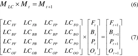
According to Eqs. (6)-(7) (Al-sharif & Pradhan, 2014; Razavi, 2014), MC model is formed by three matrices. MLC

shows the transition matrix, and Mt and Mt+1 show the stage of the system in time t0 and t1, respectively.

1

LC t t

M



M



M

1 1 1 1

FF FB FP FO t t

BF BB BP BO t t

PF PB PP PO t t

OF OB OP OO t t

LC LC LC LC F F

LC LC LC LC B B

LC LC LC LC P P

LC LC LC LC O O

                    _{ }                    (7)

where F, B, P, and O depict the Farmlands, Buildings, Parks, and Open lands land use classes, respectively. LCFB shows the probability of change from land use class B at time t to land use class F at time t+1. Ft, Bt, Pt, and Ot show the existing pixels in land use F, B, P, and O at time t. 2.1.3 Multi Objective Land Allocation

In simulation of multiple land use change issues, it is necessary to find a method for solving the allocation problems for the cases with conflicted objectives, i.e., land uses. In these cases, the MOLA procedure can solve the problems by finding the suitable areas for each objective (García-Frapolli et al. , 2007). This method can find suitable lands for each land use class based on available information from the land use suitability map, i.e., a TPM, and the value of assigned area. MOLA finds suitable areas for each objective and solves the allocation problems by considering the concept of minimum distance to ideal points. Therefore, at first, MOLA forms a matrix at the same size with the study area based on the TPM of each objective. Each pixel in this matrix has two elements in two dimensional spaces; i

and j, which are defined as objective 1 and 2 TPM’s value.

Using this process, MOLA finds the ideal point for each objective, which is a point that is maximally suitable for one objective and minimally suitable for all other objectives (in multi-dimensional space). Then, the decision line i.e., a hyper-plane in multi-dimensional space, is achieved by considering the concept of minimum distance to ideal points (Figure 3).

,

(

),

j i i j j i

O



f



OW



b

,

(

),

k j j k k j

38 Figure 3. Decision space (Eastman et al, 1998)

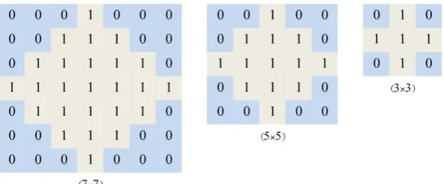
Figure 4. Three neighborhood filters

This distance is defined as the difference between each pixel’s value and ideal point’s value in TPM (Eastman et al., 1998). According to Figure 3, this line divides the disputed area into two parts. The sub-line area in disputed area belongs to objective 1 and the top-line area in disputed area belongs to objective 2. Since the simulation process is applied on four land use classes, it will cause interference in spatial allocation phase. Hence, MOLA is applied to solve the problem with conflicted objectives to integrate the TPMs based on the amount of changes and to find the suitable areas for each land use class.

2.1.4 Neighborhood Concept

Proximity is one of the basic spatial elements that underlies land use changes. Areas have a higher tendency to change to a land use class when they are more near the existing areas of that class (Jenerette & Wu, 2001). Proximity can be effectively modeled using the neighborhood filter.

The mean neighborhood filter was applied in this paper because it is strange either a building would be built on the middle of farmlands or the farmlands and open lands would

be existed in the densely urban areas. Indeed, the neighborhood is a set of one or more locations that are at a given distance or have a specific relationship with a particular location. Accordingly, the mean neighborhood filter (Figure 4) was applied to the Boolean map of each land use. Then, the result matrix are multiplied to the TPM of each land use, and consequently, the value of the distant regions was lowered in the result.

The proposed method was applied in four scenarios. The difference of these scenarios was in type of their neighborhood filter: 3×3, 5×5, and 7×7 neighborhood filters were used in the first three scenarios, and in the last scenario the simulation was performed without the neighborhood filter.

2.2 Accuracy Assessment

2.2.1 ROC

38 of a class, using a Boolean image reference that shows

where that class actually exists (Pontius & Schneider, 2001). This method computes the accuracy of modeling with different thresholds. A threshold refers to the percentage of pixels in the TPM to be reclassified as 1 for comparison with the Boolean image reference. Suppose that the threshold is considered as X %. ROC will begin with the pixel which has the highest transition potential; then it reclassifies the pixel as 1 and continues down through the pixels until X % of the pixels are reclassified as 1. The

100-X % of the remaining pixels will be classified as 0. Then, this image will be compared with the Boolean image reference (Pontius & Schneider, 2001). ROC is a curve that the X axis was computed by Eq. (8) (Pontius & Schneider, 2001; Tayyebi et al., 2010) and the Y axis was computed by Eq. (9) (Pontius & Schneider, 2001; Tayyebi et al., 2010), and was extracted from Table 1 according to the specified thresholds. Thresholds have to be determined by experience or trial and error.

%

B

FalsePositive

B

D





%

A

TruePositive

A

C





where A are pixels that are predicted as expansion of class 1, i.e., one of each land-use of this study, and agree with the reference map; B are pixels that are predicted as expansion of class 1 but disagree with the reference map; C are pixels that are predicted as expansion of class 2, i.e., three other land-uses of this study, but disagree with the reference map; and finally D are pixels that are predicted as expansion of class 2 and agree with the reference map. Hence, as the number of B and C decreases, a higher accuracy of simulation will be achieved.

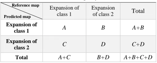
Table 1. Contingency table Reference map

Predicted map

Expansion of class 1

Expansion

of class 2 Total

Expansion of

class 1 A B A+B

Expansion of

class 2 C D C+D

Total A+C B+D A+B+C+D

Then, the ROC curve was plotted based on the thresholds and the Area Under Curve (AUC) was computed. AUC of 0.5 represents a random matching agreement between the TPM and the Boolean reference map and 1 represents the best agreement (Pontius & Schneider, 2001). In this study, the ROC was used for accuracy assessment of the predicted TPMs by the proposed ANN (Sec 2.1.1).

2.2.2 Confusion matrix

Overall accuracy (OA) and kappa index of agreement (KIA) already have been used in many studies for validating

the simulation in land use change modeling issues (Deng et al., 2008; Wang et al., 2012). These criteria reflect the match between the reference map and the simulated map. One of the advantages of the kappa index of agreement is that it uses all of the elements of confusion matrix (Robert G Pontius, 2000). The overall accuracy (OA) and the kappa index of agreement (KIA) can be obtained using Eqs. (10)-(11) (Congalton, 1991):

1

c ii i

OA





P

1 1

1

.

1

.

c c

ii iT Ti i i

c

iT Ti i

p

p

p

KIA

p

p













where i= 1,…, c shows the land use class in the study area

and Pii shows the pixels of class i in the reference map that

are also in class i in the simulated map, and Pij shows the pixels of class i in the reference map that are in class j in the simulated map, and PiT shows the sum of the pixels of class

i in the reference map and PTi shows the sum of the pixels of class i in the simulated map.

Incapability in obtaining the spatial accuracy is the main problem of OA and KIA (Robert G Pontius, 2000). In order to cover this problem, the Klocation was used. Pontius and Schneider (2001) introduced this method for the first time for spatial accuracy assessment. This criterion can be obtained using Eq. (12) (Pontius & Schneider, 2001):

1 1

1 1

.

min(

,

)

.

c c

ii iT Ti i i

location c c

iT Ti iT Ti

i i

p

p

p

K

p

p

p

p

   















OA, KIA, and Klocation change between 0 and 1 in which 1 means a higher accuracy. A KIA value less than 0.4 shows the weakness of simulation and a value more than 0.8 shows the power of simulation (Robert G Pontius, 2000).

2.3 Data set and study area

33 Table 2. Data set

Data Date Data type Resolution Source

Landsat images of TM and ETM+

2002, 2008,

2014 Raster 30 m USGS

1

Tehran’s roads map 2002, 2008, ₂₀₁₄ Vector Converted to raster, 30 m NCC2 Tehran’s DEM 2002 Raster 30 m NCC

Tehran’s Faults map 2002, 2008, ₂₀₁₄ Vector Converted to raster, 30 m NCC

Tehran’s Population map

2002, 2008,

2014 Vector Converted to raster, 30 m SCI

3

Tehran’s surrounding cities map

2002, 2008,

2014 Vector Converted to raster, 30 m NCC

Tehran’s surrounding villages map

2002, 2008,

2014 Vector Converted to raster, 30 m NCC

Tehran’s rivers map 2002, 2008,

2014 Vector Converted to raster, 30 m NCC 1 United States Geological Survey

2 National Cartographic Center of Iran 3 Statistical Centre of Iran

Figure 5. Study area

According to Figure 4, Tehran province is marked in red where a subset of the region is considered including Tehran and adjacent cities, namely Shahre-Rey, Eslamshahr, Pakdasht, Shahriar, Robatkarim, and Ghods.

3.RESULTS AND DISCUSSION

The proposed method of this paper can be explained in 5 sections:

(1) Performing the preprocessing operations: This section contains the land use map production, effective factors preparation, and production of dependent variable. (2) Performing ANN using the independent variables and

the dependent variable and obtaining the best architecture: In this section, at first, ANN was performed using 5% of data to obtain its best architecture. Then, the optimized ANN was applied to predict the TPMs using all available data. Finally, the

predicted TPMs were validated using the Boolean reference maps of each land use class by ROC. (3) Implementation of the Markov chain model for

quantification of the changes.

(4) Integrating the TPMs and the quantified changes by MOLA-neighborhood method in order to predict the land use map of 2014.

(5) Validation of the proposed method using confusion matrix.

3.1 Preprocessing operations

3.1.1 Land use/cover Maps

38 these images using the SVM classification method.

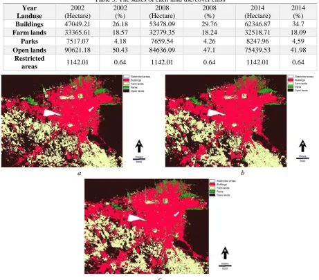
Classification was applied by the radial basis function (RBF) kernel. The achieved overall accuracy (OA) of land use classification for the 2002, 2008, and 2014 images is about 93.6 %, 94.2 %, and 95.4 % with the kappa index of agreement of 89.4 %, 90.7 %, and 91.9 %, respectively. The output of this stage is Tehran’s land use maps (Figure 6). In the study area and by considering the spatial resolution of the images, five land use classes were founded: farmlands, buildings, parks, open lands, and protected areas. The first four land use classes are changeable and the protected areas land use class is constant in simulation process. Table 3 demonstrates the states of each land use class in 2002, 2008, and 2014.

3.1.2 Independent variables

The independent variables are the variables that effect on the prediction of the future, so the ANN do not need these variables for training. According to the idea from experts and previous studies (Arsanjani et al, 2013; Tayyebi et al., 2010), four categories of factors were considered as factors affecting land use changes;

( 1

) Topography factors are DEM, slope, and aspect (Figure 7a-c). These factors are selected to involve the geographic and environmental effects of the area of interest in the simulation process .

( 2

) Socioeconomic factor is Population density (Figure 7d), which is one of the principal factors for land use changes.

( 8

) Proximity factors are distance to farm lands, distance to buildings, distance to parks, distance to open lands, distance to city’s exit nodes, distance to nearby cities, distance to faults, distance to the north (The distance of each pixel from the Northernmost pixel of each column in the study area) , distance to the west (The distance of each pixel from the Westernmost pixel of each row in the study area) , distance to rivers, distance to villages, and distance to roads (Figure 7e-p). These factors are chosen to consider the shape and the situation of the region.

(4) Boolean maps are buildings, farmlands, parks, open lands, and protected areas (Figure 7q-r4). These factors are chosen to prevent performing the simulation process in existing areas of each land use class (Boolean map of each land use is exclusively used in simulation of that land use).

Table 3. The states of each land use/cover class

Year Landuse

2002 (Hectare)

2002 (%)

2008 (Hectare)

2008 (%)

2014 (Hectare)

2014 (%)

Buildings 47049.21 26.18 53478.09 29.76 62346.87 34.7

Farm lands 33365.61 18.57 32779.35 18.24 32518.71 18.09

Parks 7517.07 4.18 7659.54 4.26 8247.96 4.59

Open lands 90621.18 50.43 84636.09 47.1 75439.53 41.98

Restricted

areas 1142.01 0.64 1142.01 0.64 1142.01 0.64

a b

c

89

a b c

d e f

g h i

j k l

m n o

81

r2 r3 r4

Datum: WGS84 Proj: UTM, Zone 39N, Scope of the case study:

NW: 51° 4' 40" E, 35° 49' 38" N. NE: 51° 36' 54" E, 35° 49' 32" N. SW: 51° 4' 38" E, 35° 29' 36" N. SE: 51° 36' 45" E, 35° 29' 31" N.

Figure 7. Independent variables for the year 2002; (a) DEM, (b) Slope, (c) Aspect, (d) Population density, (e) Distance to buildings, (f) Distance to farm lands, (g) Distance to parks, (h) Distance to open lands, (i) Distance to city’s exit nodes, (j) Distance to nearby

cities, (k) Distance to faults, (l) Distance to the north, (m) Distance to the west, (n) Distance to rivers, (o) Distance to villages, (p) Distance to roads, (q) restricted areas, (r1) Boolean map of buildings, (r2) Boolean map of farm lands, (r3) Boolean map of parks, (r4)

Boolean map of open lands.

a b

c d

Figure 8. Dependent variables, New regions of (a) Buildings, (b) Farm lands, (c) Parks, and (d) Open Lands from 2002 to 2008

Totally, 18 factors were selected for each land use simulation to fit to the model. These factors were prepared for both years 2002 and 2008 in which the factors of the former were used in training process to extract the coefficients of the variables and factors of the latter were used in prediction process.

3.1.3 Dependent variables

Unlike the Independent variables, the dependent variables are the essential needs of ANN for training. ANN needs a behavior of the past years change (Boolean map of

the new regions) of each land use class from 2002 to 2008 for training process. To obtain these maps, the Boolean maps of each land use class at the year 2002 were subtracted from those of year 2008. This operation produced Boolean maps where 1 shows the changes and 0 shows the intact areas at the period between 2002 to 2008 (Figure 8).

3.2 Transition Potential Maps production

82 class, the model was performed for buildings, farm lands,

and parks. Thus, to predict the destruction of each land use class, the method was also operated on open lands.

Altogether, ANN run four times (Figure 9); one for each land use class, and each time has two steps: (i) Training process, and (ii) Prediction process, i.e., the feed-forward process after the training process. The network was trained using the dependent variable (Figure 8) of each land use class. The independent variables in the training step were 18 factors of the year 2002. Also, 18 factors of 2008, i.e., mentioned in Section 3.1.2, were used for feed-forward process. The most important part in ANN modeling is designing a suitable structure. The designed ANN in this study includes three layers: the input, the hidden, and the output layers. Depending on the number of the independent variables, the input layer had 18 neurons. The output layer had one neuron representing the TPM. The number of neurons in hidden layer was determined using the minimum

RMSE value. In this regard, to identify the number of

neurons in hidden layer, the ANN architecture was set to 18-X-1, where 9 < X < 18 because the number of hidden layer neurons should not exceed the number of input layer and should not be less than half of that. The minimum value of the RMSE in the training process was used to decide about the optimal learning.

To prevent the over-fitting error during the training process, 5% (99830 pixels) of the data was selected for training process. Among these training data (5%), 70% was used for training and 30% was used for testing. The stopping criteria for training process define as two rules: (i) the goal of RMSE value was set to 0, (ii) the maximum training epochs was set to 1000. Once the minimal error was achieved or the training epochs are completed, the feed-forward process was applied by ANN to generate the TPM. Figure 10 represents the optimal number of the hidden layer neurons according to the minimum RMSE

value for each land use class.

Figure 9. Flowchart of the TPMs production

88 According to Figure 10, the ANN architecture was set to

18-15-1, 18-13-1, 18-15-1, and 18-15-1 for the buildings, farm lands, parks, and open lands, respectively. Figure 10 shows that, both the building and open lands classes are approximately similar in behavior. The same is true about the behavior of farmlands and parks classes because of their similar spectral properties. Figure 10 also demonstrates that the difference between the minimum and maximum values of the buildings and open lands, according to their stability, is less than those of the parks and farm lands.

The buildings, open lands, and parks were reached the minimum value of RMSE in 15 numbers of hidden neurons and the farm lands have a different behavior in a way farm lands was reached the minimum value of RMSE in 13 numbers of hidden neurons. It has the minimum accuracy compared to other land use classes that can be explained due to its fast speed of annual variability. After obtaining the optimal architecture, all of the data were introduced to ANN for feed-forward process. Figure 11 illustrates the transition potential maps (TPMs) which are the output of the optimized ANN.

The outputs of the ANN in four processes are four TPMs, one for each land use class. The accuracy of each TPM was obtained by comparing it with the Boolean

reference map of its land use class using ROC (Figure 12). According to Figure 12, the accuracy of TPMs was computed by ROC in 10 thresholds. A threshold refers to the percentage of pixels in the TPM that has the higher value than the other pixels. In each threshold, the accuracy of simulation was computed based on the existing pixels of that threshold. In simulation of multiple land use change, due to the limited number of changeable pixels, the high value pixels in TPMs are more important. Therefore, in ROC diagram, the curve which has a steeper slope in the two or three first thresholds (Figure 12; red curve) is more accurate than the curve with the lower slope (Figure 12; yellow curve), because the curve with a steeper slope obtains most of its accuracy from the high valued pixels. In addition, Figure 12 shows that the curve of the buildings land use class has a uniform change which shows that the accuracy of more suitable pixels and less suitable pixels is close to each other. The accuracy of the high value pixels (first thresholds) of the TPM of parks land use class is more than the other land use classes that it can be inferred that ANN is more successful in detecting the more suitable pixels for parks than the other land use classes. Moreover, as mentioned before, the accuracy of the TPM of the farm lands was less than the others due to its instable properties.

a b

c d

88 Figure 12. Accuracy assessment of TPMs using ROC

3.3 Quantification of the changes

In order to quantify the changes, the Markov analysis was applied to predict the amount of the changes from each land use class to another one. Historical maps of 2002 and 2008 and the temporal period (6 years) were introduced to the Markov network as inputs. Then, the amount of the changes was predicted for 2014. Table 4 illustrates the results of the Markov chain analysis.

Table 4. Markov chain model’s results in percent

2014

Land-use classes

Farm

lands Buildings Parks

Open lands

2008

Farm lands 75.1 3 2.2 19.7

Buildings 1 93.4 1 4.6

Parks 2.4 9.9 76.8 10.9

Open lands 7.8 8.6 0.8 82.8

The predicted amount of changes (Table 4) shows that the buildings land use class has the highest value of immutability (93.4 %) in comparison to those of other land use classes. In addition, the farmlands land use class was predicted as the most unstable land use class (75.1%). It was anticipated that the farmland class mostly gained from the open lands (7.8 % of open lands) due to the plant growth in open lands. Also, most of land loss of farmlands class is gained by open lands class (19.7 % of farm lands) that can be explained by the seasonal growth of plants. According to Tables 3 and 4, the predicted land gain and loss for each land use class from 2008 to 2014 is provided in Table 5.

According to Tables 4 and 5, most of land gain and loss predicted for open lands are rational considering its extent. Generally, 5490.82 ha of the area was predicted to be occupied by buildings land use class that seems reasonable due to the fast growth of Tehran.

Table 5. The predicted amount of land gain and loss for each category

Land use Land gain

(Hectare)

Land loss (Hectare)

Overall (Hectare)

Buildings 9020.37 3529.55 5490.82 gained

Farm lands 7320.23 8162.06 841.83 lost

Parks 1933.02 1777.01 156.01 gained

Open lands 9752.41 14557.41 4805 lost

3.4 Predicting land use map of 2014 in four scenarios

In order to predict land use map of 2014, the areas that were subject to change from each land use class to other classes needed to be determined. Thus, a positioning method for finding the suitable areas for each land use class had to be applied. For this purpose, the MOLA method was used. According to Section 2.1.3, MOLA can find the best areas for each objective according to its TPMs and the amount of areas that must be found for each objective. The TPMs and the amount of areas to be changed (the gained land of each land use class) were introduced to MOLA. To apply the proximity effects, in three scenarios, MOLA was combined with 3×3, 5×5, and 7×7 mean neighborhood filter. In this paper, integration of the MOLA and neighborhood filter is called the MOLA-Neighborhood method. Finally, to obtain the effects of proximity, in the last scenario, the simulation was conducted without the neighborhood filter. Figure 13 shows the flowchart of four scenarios.

3.4.1 MOLA-Neighborhood Method

88 gets a value of 1 when it is completely within the existing

areas and 0 when it is completely outside. However, when the filter moves on the boundary, its values will quickly be changed from 1 to 0. Then, the result is multiplied by the TPM for that class and the values of pixels that are far away from existing areas of that class are reduced and new TPMs are produced. Then, the new TPMs are introduced to MOLA to find the 1/n of amount of the areas to be changed

for each land use class. The results of MOLA are the predicted maps of the new areas in each epoch; then, this map overlaid by the map of 2008. The desired required areas for each class will be allocated by performing all n

epochs. Hence, the final result is the predicted map for 2014. The predicted land use maps of 2014 in four scenarios are shown Figure 14.

Figure 13. Flowchart of the four scenarios

a b

c d

88

4. Model Validation by Confusion matrix

In this section, the predicted land use maps are compared with reference map of 2014. In order to extract the accuracy of simulation from the confusion matrix, the overall accuracy, the kappa index of agreement and Klocation were employed. The accuracy of the proposed method is provided in Table 6.

Table 6. Accuracy assessment by the confusion matrix

scenario OA KIA Klocation

3×3 95.49% 92.62% 92.74%

5×5 94.02% 91.43% 91.54%

7×7 92.92% 90.61% 90.66%

non 88.79% 85.54% 85.54%

The results of the overall accuracy, the kappa index of agreement, and the Klocation illustrate the power of the proposed method in land use simulation. The results show that using neighborhood filter is a good way to increase the accuracy of simulation. Due to considering details and applying closer neighborhoods, the accuracy of the 3×3 filter is more than that of others.

The kappa index of agreement (KIA) is decomposed into two sub-components using Eq. (13) (Millington et al., 2007):

location Histo

KIA



K



K

where the KHisto defines the accuracy of abundance of land use class for the entire map and is related to quantification method, i.e., Markov Chain, and the Klocation defines the accuracy of allocation method, i.e., MOLA-Neighborhood. In the fourth scenario, the value of KIA and Klocation, which shows the accuracy of spatial allocation, are equal. Therefore, the accuracy of the spatial allocation method (MOLA- Neighborhood) and the quantification method (Markov chain) is also equal. In the best scenario (3×3 neighborhood filter), the Klocation, is slightly (0.12 %) higher than that of KIA. Thus, it can be concluded that the spatial allocation method (MOLA-Neighborhood) is more accurate than the quantification method (MC). Accordingly, it is inferred that the neighborhood filter has a positive effect in increasing the accuracy of simulation.

The accuracy achieved by the proposed method of this paper was also compared with that of the proposed method by Arsanjani et al. (2013). Arsanjani et al.'s research in 2013 is one of the latest reported accurate studies on Tehran metropolis. In both researches, the ROC and the kappa index of agreement were used to validate the model. However, in current research, the ROC value of the buildings land use class is 95.64, which is 0.34 percent greater than the ROC value of the research by Arsanjani et al. (2013). In addition, the final purpose of both researches has been the same, however the applied methods of researches are different. In this research, the proposed tuned ANN was used instead of the logistic regression and the number of independent variables of this research is more

than those by Arsanjani et al. (2013). In this regard, the additional important factors were considered in this paper including the aspect, the distance to farm lands, the distance to parks, the distance to open lands, the distance to faults, the distance to the city’s exit nodes, and the distance to villages. Furthermore, our method considers the changes for each land use class separately, while in Arsanjani et al. (2013), the simulation was only performed on the buildings land use class and was extended to the other land use classes. Moreover, in this paper, the spatial allocation was performed using neighborhood filter to consider the effects of the proximity.

Moreover, a comparison between the results of this paper and those of other papers applied on Tehran metropolis is shown in Table 7 that shows the superiority of the proposed method of this research against the other methods.

Table 7. A comparison of the results of this paper proposed method with those of some related papers

ROC KIA Reference Method 95.64 92.62 This paper ANN + MC + MOLA

80 78

[Pijanowski et al, 2010] ANN

-84.63 [Arsanjani et al 2013]

ABM+ MC

95.3 89

[Arsanjani et al 2013] LR+ MC+ CA

5. Conclusion

Integration between GIS and RS is an efficient tool to incorporate socio-economic factors in order to anticipate the future land use map. In this research, a novel method was introduced for multiple land use change simulation based on using ANN which resulted to an acceptable accuracy for Tehran metropolitan. To achieve a high accuracy in simulation process, ANN was optimized in determining the number of hidden layer’s neurons. The cycle was completed to consider the land gain and land loss for each land use class. Thus, the background of the map (open lands) was considered as one of the land use classes and was incorporated in simulation process. MC model was applied to quantify the gain and loss. This paper showed that the most land gain is for a building block that is logical because Tehran is growing fast according to its political and economic situation.

88 demonstrates the loss of farmlands in south and southwest

of the city. Thus, it requires more attention by urban planners and experts.

For future researches, this model can be combined with optimization methods such as evolutionary algorithms in factor selection stage to find the most effective factors. In this paper, the MOLA approach allocated the land use class to each pixel by the concept of minimum distance to ideal points that in future researches it can be performed by the concept of maximum neighborhood or combination of these two concepts.

Figure 15. The predicted land use map of 2020

References

Achmad, A., Hasyim, S., Dahlan, B., & Aulia, D. N. (2015). Modeling of urban growth in tsunami-prone city using logistic regression: analysis of Banda Aceh, Indonesia. Applied Geography, 62, 237-246.

Ahmed, B., & Ahmed, R. (2012). Modeling urban land cover growth dynamics using multi‑temporal satellite images: A case study of dhaka, bangladesh. ISPRS International Journal of Geo-Information, 1(1), 3-31. Al-sharif, A. A., & Pradhan, B. (2014). Monitoring and

predicting land use change in Tripoli Metropolitan City using an integrated Markov chain and cellular automata models in GIS. Arabian journal of geosciences, 7(10), 4291-4301.

Alsharif, A. A., & Pradhan, B. (2014). Urban sprawl analysis of Tripoli Metropolitan city (Libya) using remote sensing data and multivariate logistic regression model. Journal of the Indian Society of Remote Sensing, 42(1), 149-163.

Arsanjani, J. J., Helbich, M., Kainz, W., & Boloorani, A. D. (2013). Integration of logistic regression, Markov chain and cellular automata models to simulate urban expansion. International Journal of Applied Earth Observation and Geoinformation, 21, 265-275.

Bakker, M. M., Alam, S. J., van Dijk, J., & Rounsevell, M. D. (2015). Land-use change arising from rural land exchange: an agent-based simulation model. Landscape Ecology, 30(2), 273-286.

Barton, H. (1990). Local global planning. The Planner, 26, 12-15.

Basse, R. M., Omrani, H., Charif, O., Gerber, P., & Bódis, K. (2014). Land use changes modelling using advanced methods: cellular automata and artificial neural networks. The spatial and explicit representation of land cover dynamics at the cross-border region scale. Applied Geography, 53, 160-171.

Batty, M., & Xie, Y. (1994). From cells to cities. Environment and Planning B: Planning and Design, 21(7), S31-S48.

Congalton, R. G. (1991). A review of assessing the accuracy of classifications of remotely sensed data. Remote sensing of environment, 37(1), 35-46.

Deng, J., Wang, K., Deng, Y., & Qi, G. (2008). PCA‐based land‐use change detection and analysis using multitemporal and multisensor satellite data. International Journal of Remote Sensing, 29(16), 4823-4838.

Eastman, J. R., Jiang, H., & Toledano, J. (1998). Multi-criteria and multi-objective decision making for land allocation using GIS. Environment and Management, 9, 227-252.

Feng, Y., & Liu, Y. (2013). A heuristic cellular automata approach for modelling urban land-use change based on simulated annealing. International Journal of Geographical Information Science, 27(3), 449-466. Foroutan, E., & Delavar, M. (2012). Urban growth

modeling using genetic algorithms and cellular automata; A case study of Isfahan Metropolitan Area, Iran. Proceedings of the GIS Ostrava, 23-25.

García-Frapolli, E., Ayala-Orozco, B., Bonilla-Moheno, M., Espadas-Manrique, C., & Ramos-Fernández, G. (2007). Biodiversity conservation, traditional agriculture and ecotourism: Land cover/land use change projections for a natural protected area in the northeastern Yucatan Peninsula, Mexico. Landscape and urban planning, 83(2), 137-153.

García, A. M., Santé, I., Boullón, M., & Crecente, R. (2012). A comparative analysis of cellular automata models for simulation of small urban areas in Galicia, NW Spain. Computers, environment and urban systems, 36(4), 291-301.

Grekousis, G., Manetos, P., & Photis, Y. N. (2013). Modeling urban evolution using neural networks, fuzzy logic and GIS: The case of the Athens metropolitan area. Cities, 30, 193-203.

Halmy, M. W. A., Gessler, P. E., Hicke, J. A., & Salem, B. B. (2015). Land use/land cover change detection and prediction in the north-western coastal desert of Egypt using Markov-CA. Applied Geography, 63, 101-112. Hong, H., Pradhan, B., Xu, C., & Bui, D. T. (2015). Spatial

prediction of landslide hazard at the Yihuang area (China) using two-class kernel logistic regression, alternating decision tree and support vector machines. Catena, 133, 266-281.

Hosseinali, F., & Alesheikh, A. A. (2014). Assessing Urban Land-Use Expansion in Regional Scale by Developing a Multi-Agent System. The International Journal of Humanities, 20(2), 23-44.

83 Huang, B., Xie, C., Tay, R., & Wu, B. (2009).

Land-use-change modeling using unbalanced support-vector machines. Environment and Planning B: Planning and Design, 36(3), 398-416.

Jenerette, G. D., & Wu, J. (2001). Analysis and simulation of land-use change in the central Arizona–Phoenix region, USA. Landscape Ecology, 16(7), 611-626. Jiang, L., Deng, X., & Seto, K. C. (2013). The impact of

urban expansion on agricultural land use intensity in China. Land Use Policy, 35, 33-39.

Kleinbaum, D. G., Kupper, L. L., Nizam, A., & Rosenberg, E. S. (2013). Applied regression analysis and other multivariable methods: Nelson Education.

Kumar, S., Radhakrishnan, N., & Mathew, S. (2014). Land use change modelling using a Markov model and remote sensing. Geomatics, Natural Hazards and Risk, 5(2), 145-156.

Lai, T., Dragićević, S., & Schmidt, M. (2013). Integration of multicriteria evaluation and cellular automata methods for landslide simulation modelling. Geomatics, Natural Hazards and Risk, 4(4), 355-375.

Lin, C.-T. (1996). Neural fuzzy systems: a neuro-fuzzy synergism to intelligent systems: Prentice hall PTR. Lin, H., Lu, K. S., Espey, M., & Allen, J. (2005). Modeling

Urban Sprawl and Land Use Change in a Coastal Area--A Neural Network Area--Approach. Paper presented at the 2005 Annual meeting, July 24-27, Providence, RI. Lin, Y.-P., Chu, H.-J., Wu, C.-F., & Verburg, P. H. (2011).

Predictive ability of logistic regression, auto-logistic regression and neural network models in empirical land-use change modeling–a case study. International Journal of Geographical Information Science, 25(1), 65-87. Matthews, R. B., Gilbert, N. G., Roach, A., Polhill, J. G., &

Gotts, N. M. (2007). Agent-based land-use models: a review of applications. Landscape Ecology, 22(10), 1447-1459.

Millington, J. D., Perry, G. L., & Romero-Calcerrada, R. (2007). Regression techniques for examining land use/cover change: a case study of a Mediterranean landscape. Ecosystems, 10(4), 562-578.

Mitsova, D., Shuster, W., & Wang, X. (2011). A cellular automata model of land cover change to integrate urban growth with open space conservation. Landscape and urban planning, 99(2), 141-153.

Moghadam, H. S., & Helbich, M. (2013). Spatiotemporal urbanization processes in the megacity of Mumbai, India: A Markov chains-cellular automata urban growth model. Applied Geography, 40, 140-149.

Molowny-Horas, R., Basnou, C., & Pino, J. (2015). A multivariate fractional regression approach to modeling land use and cover dynamics in a Mediterranean landscape. Computers, environment and urban systems, 54, 47-55.

Munshi, T., Zuidgeest, M., Brussel, M., & van Maarseveen, M. (2014). Logistic regression and cellular automata-based modelling of retail, commercial and residential development in the city of Ahmedabad, India. Cities, 39, 68-86.

Nouri, J., Gharagozlou, A., Arjmandi, R., Faryadi, S., & Adl, M. (2014). Predicting urban land use changes using

a CA–Markov model. Arabian Journal for Science and Engineering, 39(7), 5565-5573.

Paola, J. D., & Schowengerdt, R. A. (1995). A detailed comparison of backpropagation neural network and maximum-likelihood classifiers for urban land use classification. IEEE Transactions on Geoscience and remote sensing, 33(4), 981-996.

Pijanowski, B. C., Brown, D. G., Shellito, B. A., & Manik, G. A. (2002). Using neural networks and GIS to forecast land use changes: a land transformation model. Computers, environment and urban systems, 26(6), 553-575.

Pijanowski, B. C., Tayyebi, A., Doucette, J., Pekin, B. K., Braun, D., & Plourde, J. (2014). A big data urban growth simulation at a national scale: configuring the GIS and neural network based land transformation model to run in a high performance computing (HPC) environment. Environmental Modelling & Software, 51, 250-268.

Pontius, R. G. (2000). Quantification error versus location error in comparison of categorical maps. Photogrammetric engineering and remote sensing, 66(8), 1011-1016.

Pontius, R. G., & Schneider, L. C. (2001). Land-cover change model validation by an ROC method for the Ipswich watershed, Massachusetts, USA. Agriculture, Ecosystems & Environment, 85(1), 239-248.

Porta, J., Parapar, J., Doallo, R., Rivera, F. F., Santé, I., & Crecente, R. (2013). High performance genetic algorithm for land use planning. Computers, environment and urban systems, 37, 45-58.

Rafiee, R., Mahiny, A. S., Khorasani, N., Darvishsefat, A. A., & Danekar, A. (2009). Simulating urban growth in Mashad City, Iran through the SLEUTH model (UGM). Cities, 26(1), 19-26.

Randolph, J. (2004). Environmental land use planning and management: Island Press.

Razavi, B. S. (2014). Predicting the trend of land use changes using artificial neural network and markov chain model (case study: Kermanshah City). Research Journal of Environmental and Earth Sciences, 6(4), 215-226.

Rendana, M., Rahim, S. A., Idris, W. M. R., Lihan, T., & Rahman, Z. A. (2015). CA-Markov for Predicting Land Use Changes in Tropical Catchment Area: A Case Study in Cameron Highland, Malaysia. Journal of Applied Sciences, 15(4), 689.

Schneider, L. C., & Pontius, R. G. (2001). Modeling land-use change in the Ipswich watershed, Massachland-usetts, USA. Agriculture, Ecosystems & Environment, 85(1), 83-94.

SCI. (2010). www. Amar.org.ir.

Shafizadeh-Moghadam, H., Hagenauer, J., Farajzadeh, M., & Helbich, M. (2015). Performance analysis of radial basis function networks and multi-layer perceptron networks in modeling urban change: a case study. International Journal of Geographical Information Science, 29(4), 606-623.

88 and Tianjin: A case study of Zhangjiakou city, Hebei

Province. Journal of Geographical Sciences, 26(3), 272-296.

Tan, R., Liu, Y., Zhou, K., Jiao, L., & Tang, W. (2015). A game-theory based agent-cellular model for use in urban growth simulation: A case study of the rapidly urbanizing Wuhan area of central China. Computers, environment and urban systems, 49, 15-29.

Tayyebi, A., Delavar, M. R., Yazdanpanah, M. J., Pijanowski, B. C., Saeedi, S., & Tayyebi, A. H. (2010). A spatial logistic regression model for simulating land use patterns: a case study of the Shiraz Metropolitan area of Iran Advances in earth observation of global change (pp. 27-42): Springer.

Tayyebi, A., Perry, P. C., & Tayyebi, A. H. (2014). Predicting the expansion of an urban boundary using spatial logistic regression and hybrid raster–vector routines with remote sensing and GIS. International Journal of Geographical Information Science, 28(4), 639-659.

Tayyebi, A. H., Tayyebi, A., & Khanna, N. (2014). Assessing uncertainty dimensions in land-use change models: using swap and multiplicative error models for injecting attribute and positional errors in spatial data. International Journal of Remote Sensing, 35(1), 149-170.

Wang, S., Zheng, X., & Zang, X. (2012). Accuracy assessments of land use change simulation based on Markov-cellular automata model. Procedia Environmental Sciences, 13, 1238-1245.

Wang, Y., & Li, S. (2011). Simulating multiple class urban land-use/cover changes by RBFN-based CA model. Computers & geosciences, 37(2), 111-121.

White, R., & Engelen, G. (1993). Cellular automata and fractal urban form: a cellular modelling approach to the evolution of urban land-use patterns. Environment and planning A, 25(8), 1175-1199.

Xia, T., Wu, W., Zhou, Q., Verburg, P. H., Yu, Q., Yang, P., & Ye, L. (2016). Model-based analysis of spatio-temporal changes in land use in Northeast China. Journal of Geographical Sciences, 26(2), 171-187. Xie, C. (2006). Support vector machines for land use

change modeling. UCGE Reports, Calgary.

Yan, B., Fang, N., Zhang, P., & Shi, Z. (2013). Impacts of land use change on watershed streamflow and sediment yield: an assessment using hydrologic modelling and partial least squares regression. Journal of Hydrology, 484, 26-37.

Yang, X., Chen, R., & Zheng, X. (2016). Simulating land use change by integrating ANN-CA model and landscape pattern indices. Geomatics, Natural Hazards and Risk, 7(3), 918-932.

Yang, X., Zhao, Y., Chen, R., & Zheng, X. (2016). Simulating land use change by integrating landscape metrics into ANN-CA in a new way. Frontiers of Earth Science, 10(2), 245-252.