ON-LINE PARAMETER INTERVAL ESTIMATION USING RECURSIVE LEAST SQUARES

INTERNATIONAL JOURNAL OF ADAPTIVE CONTROL AND SIGNAL PROCESSING, VOL. 8, 61-72 (1994)

ON-LINE PARAMETER INTERVAL ESTIMATION USING

RECURSIVE LEAST SQUARES

PER-OLOF GUTMAN

Faculty of Agricultural Engineering, Technion

-

Israel Institute of Technology, Haifa 32000, Israel

SUMMARY

A bank of recursive least-squares (RLS) estimators is proposed for the estimation of the uncertainty intervals of the parameters of an equation error model (or RLS model) where the equation error is assumed t o lie between known upper and lower bounds. It is shown that the off-line least-squares method gives the maximum and minimum parameter values that could have produced the recorded input-output sequence. By modifying the RLS estimtor in two ways, it is possible to recursively compute inner and outer bounds of the uncertainty intergals. It is shown that the inner bound is asymptotically tight.

KEY WORDS Least-squares estimation Parameter estimation Recursive least squares

Set membership estimation

1. INTRODUCTION

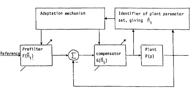
The motivation of this paper is a desire to make the Horowitz robust control design method' adaptive. In the Horowitz method it is suitable to describe the plant uncertainty as transfer function value sets or alternatively as plant parameter sets or intervals. The resulting controller consists of a linear time-invariant feedback compensator and prefilter. In Reference 2 a method was suggested of how to change on-line the parameters of such a robust controller when it becomes known that the plant parameters each belong to a smaller interval than the original interval on which the design was based. Combined with a parameter interval estimator, an adaptive robust controller is created based on the principle of robust certainty equivalence3 (see Figure 1). In Reference 3 an example from Reference 2 is simulated with essentially the parameter interval estimator presented here. Conventional adaptive controllers are, on the other hand, in general designed according to the certainty equivalence4 principle, whereby the adaptation is based on a point estimate of the parameter vector.

The vast literature on the parameter set or set membership estimation problem is covered in several informative A most attractive method is the one developed by Walter and Piet-Lahanier, which gives an exact polyhedral description of the feasible parameter set. One might even surmise that for most linear problems it obviates the need for any other method. However, approximants have been proposed such as bounding ellipsoids. '*lo Therefore the small idea in this paper, originally presented at an IFAC conference, l 1 might

hopefully evoke some interest.

It is shown that a bank of modified recursive least-squares (RLS) estimators, under weak assumptions, gives asymptotically tight inner bounds of the feasible parameter intervals for linear equation error (RLS) models. Another variation yields non-tight outer bounds. Hence the method belongs to the class of inner-bounding and outer-bounding orthotopic

CCC 0890-6327/94/01006 1 - 1 2

62

r

Adapt a t i on mec han i sin

P . - 0 . GUTMAN

I d e n t i f i e r o f p l a n t p a r a m e t e r

+- s e t , giving ?.

[image:2.576.120.453.66.221.2]

R e f e r e n c e

Figure 1 . Block diagram of control system with adaptive-feedback and prefilter control. p is the plant parameter vector. fI, is the plant parameter uncertainty set estimate. l l i is the plant parameter set on which the design is based,

with f i i 1

fr,

estimators. 6 ~ 1 2 The estimator of Kosut, l 3 where parameter sets of an output error model with unstructured uncertainty are estimated via the discrete Fourier transform (DFT) of the input-output sequences, bears some resemblance to the one analysed here.

Since estimates of value sets in the frequency domain would also serve the initially stated purpose, l4 a few relevant references could be mentioned: Goodwin and Salgado” estimate

value sets directly via a probabilistic RLS approach, while LaMaire et al. l6 and Wahlberg and

Ljung

*’

calculate error-bounding functions in the frequency domain.

The paper is organized as follows. In Section 2 the off-line and on-line algorithms are presented and analysed. Section 3 contains three simulated examples. In Section 4 the proposed algorithm is related to other methods and various advantages and disadvantages are discussed.

r

P l a n t compensator

P r e f i l t e r

2 FCGi!

2. ESTIMATION OF PARAMETER INTERVALS

2.1. Off-line parameter interval estimates

Among various algorithms for plant parameter estimation 18s19 and recursive estimation20,21

we find the popular least squares (LS) and the recursive least squares (RLS) and its relatives. In the above references, conditions on the model, input sequence and noise sequence are stated for the RLS estimates to converge asymptotically, with and without bias with respect to the true parameter values.

The LS and RLS algorithms will be the point of departure in this paper. Let the ‘true’ process be

(1)

where 8 = (a1

...

a,, bl

...

b,)T is the parameter vector and (p(t) = [ - y ( t

-

1)

...

- y ( t - n ) u(t

-

1)

...

u(t

-

m)] is the vector of measured lagged input-output data. ( u ( t ) ) is the measured input signal and ( y ( t ) ) is the measured output signal. t = 1 , 2 , 3 ,

...

is the running sample index. The equation error ( v ( t ) l includes all effects of measurement noises, mismodelling, disturbances and other uncertainties in the given description of the data. Then

ON-LINE PARAMETER INTERVAL ESTIMATION

the LS estimates eLS(N) at time t =

N

is given byi8

Introduce the matrix

The pure RLS estimate e ( t ) is given by''

e ( t ) = e(t

-

1)

+

P ( t ) p ( t ) [ y ( t ) -

e(r

-

l)=cp(t)l (4)

For suitable initial conditions of the RLS algorithm"

e ( t )

= eLS(t) and P ( t ) = R(t)-'/t for all t; for any positive definite P(O), d ( t ) and P ( t ) converge to e L S ( t ) and R ( t ) - ' / t respectively. For constant 0 the estimate

d ( t )

converges to 0 under ideal conditions." Also under ideal conditionsi8 P ( t ) is the normalized variance of the estimate XoP(t) = E [ [ & t )

-

01 [& t )

-

elT), where XO is the variance of v ( t ) .

Like the pure RLS estimator, most algorithms give point and variance estimates only. Under ideal conditions the variance matrix P ( t ) of the RLS estimator could be used for estimating a likely parameter set. In practice, however, the updating of P ( t ) in ( 5 ) is modified to include e.g. a forgetting factor, or dead zone, or devices to keep e.g. tr[P(t)] constant, or other control of P(t),22,'3 e.g. in order to enhance the tracking ability of the estimator. Then P ( t )

does not represent the variance of the estimate. It will be a ~ ~ u m that the e d ~ ~ ~ ~ ~ ~ ~ ~ ~ ~ ~ ~ ~ ~ ~

equation error in (1) is bounded, i.e.

I

v(t)l < V ( t )

<

V V t (6)

with V ( t ) or V known. It will now be shown how this assumption may be used to compute parameter interval bounds.

It is easy to show l8 that the LS estimation error 8 ( N ) = eLS(N) - 6 is given by

&N)=

[ R ( N ) ] - ' _f_

2

p ( t ) v ( t ) (7)

N

t = i

Comparing with (2), notice that with ( v ( t ) ) given, (7) can be implemented in the recursive form

(4),

(9,

with v ( t ) replacing y ( t ) and

6

replacing

8

in

(4),

with P ( t ) given by ( 5 ) :

e'(t) = e(t

-

1) + P(t)Tcp(t) v ( t )

-

e(t - l)=cp(t)l (8)

The sequence (v(t)j is, however, not known and hence the estimation error cannot be found. It is, however, easy to dream up the worst possible equation error sequence i u ( t ) ) satisfying

(6) that will yield a maximal upper bound for

I

8(N)I. For i = 1,2,

...,

n

+

m

let

v i ( t ) = V(t)sign([R(N)] -'cp(t))i (9)

64 P.-0. GUTMAN

or equivalently

e F S ( N ) - E i ( i , N )

<

f3i

<

d F S ( N )

+

E i ( i , N )

MI = (0:

8 f S ( t )

-

Ej(i, t )

<

f3i

6

d f S ( t )

+

Ei(i, t ) Vi, Vt

<

N )

(12)

Define

(13)

Clearly MI defines the maximal parameter intervals in which those parameter components are to be found that are able to produce the recorded input-output sequence assuming the model

(11, (6).

Assume18 that the input ( u ( t ) ] is quasi-stationary such that R ( N ) -+ R*, as N --* m. Assume further that all elements of p ( t ) are bounded and quasi-stationary. Then

(1/N) E z l p ( t ) u i ( t ) + h: V i as N -+ m. Hence E ( i , N ) converges as N - t a.

Equations (9)-(11) are suitable for off-line implementation. For on-line use P ( t ) can be computed using (5), while the expanding matrix cP(t) = [(p(l)p(2)

...

p ( t ) ] has to be saved in order to compute uj(t). This may constitute an unacceptable memory burden. The next subsection will treat on-line approximations of (9) and (10).

It may be noticed that V in (6) may be estimated from the residual. Assume that an LS parameter estimate has been computed, & N ) . Compute the residual

~ ( t ) = u ( t )

-

(p(t)T6(N), t

<

N (14)

Then maxt

I

e ( t )

I

may serve as an estimate of V. It is expected that this estimate will be conservative, since 8 ( N ) is in general a biased estimate of 0.

2.2. On-line parameter interval estimates

parameter intervals in essentially the following way. For each i let

In Algorithm 2 of Reference 3 a bank of RLS estimators was suggested to estimate

Comparing with (9) and (lo), it is clear that D j ( i , N )

<

E j ( i , N ) , since ( v j ( t ) ] was chosen to maximize Ei ( i , N). However, (15) is suitable for recursive implementation via (8), with P ( t ) given by ( 5 ) :

(16)

The selection of Y in (15a) simply means a 'local in t' maximization of D i ( i , N ) in (15b) and (16), in contrast with the ' a posteriori at t = N' maximization of E i ( i , N ) in (10) via the selection of u in (9).

Assume as above that R ( N ) - + R * as N - + m. Then for every i, v i ( t ) -+ v i ( t ) and hence D i ( i , t ) - + E i ( i , t ) as t + m .

We conclude that Di (i, t ) is a lower, progressively closer bound for the ith parameter interval extension Ej (i, t ) . An upper bound for Ei

(i,

t )

can also be found.

Let M = (mij] be a matrix whose elements are mij. Define abs(M)=

[I

m i j i ) . Let the

definition also hold for vectors. Let

D ( i , t ) = D(i, t - 1)

+

P ( t ) p ( t ) [ v i ( t )

-

D(i, t

-

l)'p(t)] Vi

l N

N t = l

ON-LINE PARAMETER INTERVAL ESTIMATION 65

Comparing with ( l o ) , it is immediately clear that Ei(i, N )

<

F i ( N ) , since all elements on the right-hand side of (17) are non-negative. Moreover, if it is assumed as above that R ( N ) -+ R*

as N -+ m, then of course abs( [R(N)] -') also converges. As above, assume further that all elements of ~ ( t ) are bounded and quasi-stationary. Then (l/N) X E l abs(cp(t)) V ( t ) converges. Hence F ( N ) converges as N

-,

a.

The convergence limit of F ( N ) does not seem to be possible to find without additional specific assumptions which have to be validated in each particular case. Clearly, from (10) and

(17), 0

<

E i ( i , N ) - E i ( i , N - 1) < F i ( N ) - F i ( N - 1). Assume, for instance, that when

N -+ co, E i E j ( i , N )

-

E j ( i , N - l)] = x E [ F j ( N )

-

F i ( N - l ) ) , where E f * ] means expected value and x E [ 0,1]. Then, with FO some constant vector, F ( N ) -+ Ei (i, N ) / x

+

FO as N -+ 00.

The computation of F ( N ) is easily made recursive:

W )

=

W

-

1 )

+

abs(cp(0) U t ) ( W

F ( t ) = abs(W))rC/(t) (18b)

with P ( t ) given by ( 5 ) and $ ( O ) = 0.

2.3. Summary

equation error (6), the maximally possible parameter intervals (12) for each parameter B i ,

From the recorded input-output data and an assumed RLS model ( 1 ) with bounded

(19)

have been computed, with E ( i , N ) given by (9) and (10). Since E ( i , N ) is not conveniently computed in a recursive way, recursively computable inner, D(i, t ) in (15a) and (16), and outer,

F ( t ) in (18), bounds were found:

(20)

Under weak assumptions D ( i , N ) , E ( i , N ) and F ( N ) converge to their respective limits as

N -+ 00, with D(i, N ) and E(i, N ) sharing the same limit.

B i E [SFs(N)

-

E j ( i , N ) , B f S ( N )

+

E i ( i , N ) ]

Di

(i, N )

6

Ei (i, N )

<

Fj ( N )

3. EXAMPLES

Example I

Let the 'true' process model be given by

y ( t ) = aly(t - 1 )

+

blu(t

-

1 )

+

u ( t

-

1 )

where 0 = (a1 bl)' = (0.5 1)' is the parameter vector and ~ ( t ) = [ y ( t - 1 ) u ( t

-

l)] is the vector of measured lagged input-output data. The input signal ( u ( t ) ) was chosen to be a uniformly distributed random variable in [ - 1 , 1 ] independent for each t. y(0) was set to zero. The equation error [ u ( t ) ) was chosen to be a uniformly distributed random variable in [ - 1 , 1 ]

independent for each t and independent of ( ~ ( t ) ) . It is assumed known that in ( 6 )

V ( t ) =

v =

1 .

The system was simulated for t = 1,2,

. .

.,

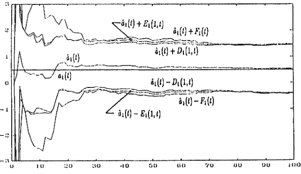
100. For one particular simulation the LS estimate

( 2 ) or (4) became $(loo) = (0.5341 0-9575)T. Such a good estimate is expected because of the nature of ( u ( t ) ) and ( ~ ( t ) ) .

From (10) E(1, t ) and E(2, t ) were computed, with the final values E 1 ( l , 100) = 0,9317 and

66 P.-0. GUTMAN

(16) D(1, t) and D(2, t) were computed, with the final values D1(1,100) = 0.9102 and

D(2,lOO) = 1.5974. From (18) F ( t ) was computed, with the final values Fl(100) = 0.9369 and

61 ( t ) , 61 ( t ) ? El (1, t ) , 81 ( t ) k DI (1 , t) and 61 (t) k Fl (t) are displayed in Figure 2.

61

(t),

&(t) 2 &(2, t ) , &(t) rt D2(2, t) and 61(t) ? F z ( t ) are displayed in Figure 3. From the figures it is seen that (20) holds and that D(i, t) seems to be a good approximation of E(i, t) at all times, while F ( t ) is satisfactory at ‘steady state’ for t

>

30.

Although the computed parameter intervals may seem exaggerated, there do exist worst-case parameter combinations, with either a1 or bl at the endpoint of its respective interval, that may yield the observed data. In the simulated case, not both a1 and bl may be at an interval endpoint. This is reflected by the low values of D2 (1,100) = 0.03072 and

Di

(2,100) = 0-0439.

Sharper bounds might be obtained by a linear transformation of the ( y ( t ) u ( t - 1)) space, yielding estimates of linear combinations of a1 and bl.

Fi(100) = 1 *6360.

O I Y ‘

[image:6.576.136.443.250.428.2]

I 1 I 0 “ 0 :lo dl0 5 0 (111 -/o 00 00 100

ON-LINE PARAMETER INTERVAL ESTIMATION 67

Example 2

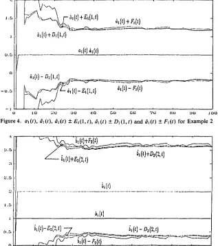
This example is extreme in the sense that u ( t ) is highly dependent on cp(t).

The process is the same as in Example 1 , equation (21), with the exception that ( v ( t ) ) = ( u ( t ) ) . One simulation was performed. The RLS estimate is very good in the sense that the prediction error is zero: &loo) = (0-5 2 ~ 0 ) ~ . The knowledge of the size of u ( t ) gives, however, the opportunity to find other parameter values that could have generated the data.

E(1, t ) and E(2, t ) were computed, with the final values E1(1,100) = 0.6880 and

E2(2,100)= 1.6257. Consequently, U I E [Om5 f 0-68801 and bl E [2.0 f 1.62571. The large parameter intervals are justified; the 'correct' 8 is found in the estimated parameter set. D(1, t ) and D(2, t ) were computed, with the final values Dl(1,lOO) = 0.6815 and Dz(2,lOO) = 1.6089.

F ( t ) was computed, with the final values Fl(100) = 0.6933 and Fz(100) = 1-6384.

& ( t ) , cil(t) k El(1, t ) , &(t) -I- Dl(1, t ) and & ( t ) k Fl(t) are displayed in Figure 4. & ( t ) , & ( t ) k Ez(2, t ) , & ( t ) k D2(2, t ) and & ( t )

+-

Fz(t) are displayed in Figure 5 . From the figures it is seen that (20) holds and that D(i, t ) and F ( t ) seems to be a good approximation of E(i, t ) .

0 LO "0 30 40 G O 6 0 7 0 I I U 3 0 100

[image:7.576.132.449.268.626.2]

68 P . - 0 . GUTMAN

Example 3

In this example the more ‘realistic’ situation of a first-order continuous-time model with stepwise jumping parameters is investigated. The example is adapted from Reference 3.

To represent the parameter intervals, the inner bounds D(i, t ) are computed with a bank of modified RLS estimatorsz4 of a type that could be used in practice. An aim of this example

is to illustrate how the parameter interval estimator fares together with modified RLS. The equations of the modified RLS identifier are

0 if y t = 0 or let

I

<

WI 1 otherwise

T yr = pt PI- lcpf

Pt=Pr-i-Pt-icprp:Pt-i(l

-

w t / I e t l ) + ( l -~)f‘r-i (22f)

This algorithm disregards redundant data and prevents Pr -+ 0 when such data are received.

( 2 3 4

(23b) Consider the first-order dynamic system as

a

function of time T:

i(7) = - J Z ( T )

+

k U ( T ) Y (7) = z ( 7 )

+

n (7)

where

I

n ( ~ )

I

<

0.01 is a uniformly distributed measurement noise. The unknown parameters

k and p , which occasionally change stepwise, have to be estimated. A priori parameter bounds are kE [ 1,101 and p E [0-5,3]. By lowpass filteringz5 y ( ~ ) and u ( T ) , one gets an identification model (l), with

I

ut

1

bounded, whose parameter vector 0 is invertibly related to k and p . Let C l ( 7 ) = - (1/C)Ui(7)

+

( l / C ) U ( T ) (24a)

j l ( T ) = -(l/C)Y1(7)

+

(l/C)Y(T) (24b)

Y(7) = -aly1(7)

+

blUl(7)

+

u ( T ) (25)

with a l = p c - 1, b l = k c , ~ ( ~ ) = n ( 7 ) + a l n l ( ~ ) and &(7)= - ( l / c ) n ~ ( ~ ) + ( l / c ) n ( ~ ) . Clearly

I

nl(7)

I

<

max(n(T)), since n l ( 7 ) equals n ( ~ ) transmitted through

a

first-order filter. Using

the lower limit of p , we get that m a x ) a l

I

= 10.5 xO.1 - 11 = 0 - 9 5 and

I

U(T)

I

<

max

I

n ( ~ ) ( 1

+

I

al

I)/

= 0.0195. Notice that (25) is valid at all times 7. Hence y(7),

y l (7) and ~ ( 7 ) may be sampled at arbitrary times, for instance with non-uniform sampling periods. Let 8 = (al b t ) T and pt = [ - y l ( r ) u1 (T)] T, where the index t is the running sample index as in (1).

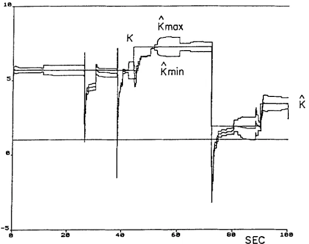
The system is excited with a square wave input U ( T ) (see Figure 6 ) . k and p are changing with random steps at random times according to Figures 7 and 8 respectively. Because of the parameter changes, the output y ( 7 ) varies wildly (see Figure 6).

The modified RLS identifier (22) was used as a conventional point estimator t o estimate

( k , p )

in the following manner. Wr was used as a tuning parameter and set t o 0.013. In (22d)

ON-LINE PARAMETER INTERVAL ESTIMATION

1

69

15.,

10

5

0

- 5

- 1 0

[image:9.576.134.448.366.614.2]

- 1 5 * 0 . 1 2 5 . 5 0 7 5 . SEC 1 0 0 .

70 P . - 0 . GUTMAN

-2 ₁

lee

SEC

e ze 4e 68 80

Figure 8. The true parameter p and its a priori bounds, the point estimate fi and the estimates of the interval bounds

@,,,in and fimnr for Example 3

To essentially compute D(i, t ) , i = 1,2, for the interval bounds Lmin, Gmax, &in and Bmax,

two copies of (22a) were used with

8,

replaced by D(i, t ) , i = 1,2, and et replaced by

[image:10.576.131.444.66.327.2]

v i ( t )

-

D(i, t

-

l P p ( t ) respectively. See (16). v i ( t ) was computed according to (15a) with

[ R ( t ) ] - ' replaced by t P ( t ) , with P ( t ) taken from (22f). Y ( t ) was set to W t +

maxi

v ( 7 )

I

= 0.0325 to account for both the equation error U(T) in (25) and the dead zone

Wt in (22).

and the a priori

bounds are plotted, and in Figure 8, where p , @, f i m i n , Bmax and the a priori bounds are displayed. The estimates were not projected into the

a

priori given parameter set. We observe that the estimates converge to their approximate steady state values after steps in u ( T ) , i.e. when u ( 7 ) excites the system. The point estimate

(&a)

is of good quality but exhibits an occasional bias. In most cases the parameter interval estimates include the true parameters when steady state has been reached. We observe that there is cross-talk between the parameter estimates: a jump in p influences

h?,

Emin and

kmax

and (less so) vice versa. It should be remarked that the upper parameter interval estimate F from (18), with P(1) taken from (22) and V ( t ) as above, diverged. This is due to the fact that P ( t )

+

0 in (22).

If the parameter interval estimates in this example are to be used for the adaptation of a robust controller,' then the robust controller should be based on the full a priori parameter uncertainty whenever an abrupt parameter change is sensed. Only when the estimator has reached steady state could adaptation take place using the interval estimates with appropriate safety margins.

ON-LINE PARAMETER INTERVAL ESTIMATION 71

4. CONCLUSIONS

From the recorded input-output data and an assumed RLS model with bounded equation error, the feasible parameter intervals for each parameter B i , B i E [ 8 F S ( N )

-

E i ( i , N ) , 8 k S ( N )

+

Ei

(i,

N ) ] , have been computed. Since E(i, N ) is not conveniently computed in a recursive way, a recursively computable inner, D(i,

N),

and outer, F(N), bounding was found:

Di

(i,

N )

<

Ei ( i , N )

<

Fi ( N ) . Under weak assumptions D(i, N), E(i, N ) and F ( N ) converge to their respective limits as N + OQ, with D(i, N ) and E ( i , N ) sharing the same limit.

It should be pointed out that

Ei

(i,

N)

exactly describes the feasible parameter interval in the worst-case sense: there exists a feasible equation error sequence that could have produced the input-output data with the parameter value belonging to the interval. Moreover, Di(i, N ) is an asymptotically exact inner bound of E i ( i , N ) . Hence it is believed that a contribution of this paper is the development of orthotopic6”’ inner bounding.

The proposed algorithm is obviously not a special case of projecting ellipsoidal inner and outer boundings 5-7*9,10 along the parameter axes, since the covariance matrix P ( t ) is not used

for the interval estimate. Instead, a specially constructed, worst-case equation error sequence is employed. Moreover, it has been demonstrated that bounding ellipsoids are very ~ r u d e ; ~ ’ ~ in particular, the inner ellipsoid tends to vanish. Our inner bound Di(i, N), is asymptotically exact.

The weak point of the algorithm is the convergence limit of F i ( N ) , which in general does not equal the limit of Ei

(i,

N). Under additional assumptions on the data the distance between the limits may be established. The simulations of Examples 1 and 2 indicate, however, that there are cases when the limits are close.

The algorithm possesses the same tracking ability as the RLS on which it is based, since the estimated intervals are centred around their respective point estimates. However, the interval estimates may be unreliable during transients (Example 3).

In most cases methods giving an exact description’ of the feasible parameter set should be preferable. However, for a practitioner who already has a well-oiled RLS or one of its cousins running in his system, only a marginal additional effort is necessary to include the parameter set estimator proposed here. Our algorithm can also be seen as a small contribution to combining statistical and set membership estimators.

Finally, it could be argued that the analysis in this paper is rather routine and straightforward. Well, is it not nice that sometimes it is possible to get interesting, useful and novel results with easy means?

ACKNOWLEDGEMENTS

This research was supported by the Technion VPR Fund-Alexander Goldberg Memorial Research and by the Swedish Board for Technical Development, NUTEK. The comments of an anonymous and humorous reviewer were very much appreciated.

REFERENCES

1 . Horowitz, I . M., and M. Sidi, ‘Synthesis of feedback systems with large plant ignorance for prescribed time domain tolerances’, fnt. J. Contra/, 16, 287-309 (1972).

2. Yaniv, O., P. 0. Gutman and L. Neumann, ‘An algorithm for the adaptation of a robust controller to reduced plant uncertainty’, Automatica, 26, 709-720 (1990).

12 P.-0. GUTMAN

4. Astrom, K. J., and B. Wittenmark, Adaptive Control, Addison-Wesley, Reading, MA, 1989.

5 . Milanese, M., and A. Vicino, ‘Estimation theory for dynamic systems with unknown but bounded uncertainty: an overview’, Prepr. 9th IFAC/ IFORS Symp. on Identification and System Parameter Estimation, Budapest,

6 . Walter, E., and H. Piet-Lahanier, ‘Estimation of parameter bounds from bounded-error data: a survey’, Math.

7. Norton, J. P., ‘Identification and application of bounded parameter models’, Aufomatica, 23, 497-507 (1987). 8. Walter, E., and H. Piet-Lahanier, ‘Exact recursive description of the feasible parameter set for bounded-error

models’, IEEE Trans. Automatic Control, AC-34, 91 1-915 (1989).

9. Fogel, E., and Y. F. Huang, ‘On the value of information in system identification - bounded noise case’,

Automafica, 18, 229-238 (1982).

10. Dasgupta, S., and Y. F. Huang, ‘Asymptotically convergent modified recursive least squares with data dependent updating and forgetting factor for systems with bounded noise’, IEEE Trans. Info. Theory, IT-33, 383-392 (1987).

11. Gutman, P . O., ‘On-line identification of transfer function value sets’, Prepr. 9th IFAC/ IFORS Symp. on Identijcation and Systems Parameter Estimation, Budapest, 1991, pp. 758-762.

12. Milanese, M., and G. Belforte, ‘Estimation theory and uncertainty intervals evaluation in presence of unknown but bounded errors: linear families of models and estimators’, IEEE Trans. Automatic Control, AC-27, 408-414 (1982).

13. Kosut, R. L., ‘Adaptive control via parameter set estimation’, Int. J. Adapl. Control Signal Process, 2, 371-400 (1988).

14. Gevers, M., ‘Connecting identification and adaptive control: a new challenge’, Prepr. 9th IFACl IFORS Symp.

on Identification and System Parameter Estimation, Budapest, 1991, pp. 1-10.

15. Goodwin, G. C., and M. E. Salgado, ‘A stochastic embedding approach for quantifying uncertainty in the estimation of restricted complexity models’, Int. J. Adapt. Control Signal Process., 3 , 333-356 (1990). 16. LaMaire, R. O., L. Valavani, M. Athans and G . Stein, ‘A frequency domain estimator for use in adaptive control

systems’, Automatica, 21, 23-38 (1991).

17. Wahlberg, B., and L. Ljung, ‘Hard frequency-domain model error bounds from least-squares like identification techniques’, IEEE Trans. Automatic Control, AC-37, 900-912 (1992).

18. Ljung, L., System Identijcation: Theory f o r the User, Prentice-Hall International, Englewood Cliffs, NJ, 1987. 19. Soderstrom, T., and P. Stoica, System Identification, Prentice-Hall International, Hemel Hempstead, 20. Ljung, L., and T. Soderstrom, Theory and Practice of Recursive Identi$cation, MIT Press, Cambridge, MA, 21. Goodwin, G. C., and K. S. Sin, Adaptive Filtering, Prediction, and Control, Prentice-Hall, Englewood Cliffs, 22. Middleton, R. H., G. C. Goodwin, D. J . Hill and D. Q. Mayne, ‘Design issues in adaptive control’, IEEE Trans.

23. Hagglund, T., ‘New estimation techniques for adaptive control’, Ph.D. Thesis, Department of Automatic 24. Canudas de Wit, C. A., ‘Commande adaptatives pour des systemes partiallement connus’, Ph.D. Thesis,

25. Johansson, R., ‘Identification of continuous time dynamic systems’, CODEN: LUTFDZI(TFRT-7318) 11-291,

1991, pp. 859-867.

Comput. Simul., 32, 449-468 (1990).

Hertfordshire, U.K., 1989. 1983.

NJ, 1984.

Automatic Control, AC-33, 50-58 (1988). Control, Lund Institute of Technology, 1983.