R E S E A R C H
Open Access
Target parameter estimation for spatial
and temporal formulations in MIMO radars
using compressive sensing
Hussain Ali
1*, Sajid Ahmed
2, Tareq Y. Al-Naffouri
2, Mohammad S. Sharawi
1and Mohamed-S Alouini
2Abstract
Conventional algorithms used for parameter estimation in colocated multiple-input-multiple-output (MIMO) radars require the inversion of the covariance matrix of the received spatial samples. In these algorithms, the number of received snapshots should be at least equal to the size of the covariance matrix. For large size MIMO antenna arrays, the inversion of the covariance matrix becomes computationally very expensive. Compressive sensing (CS) algorithms which do not require the inversion of the complete covariance matrix can be used for parameter estimation with fewer number of received snapshots. In this work, it is shown that the spatial formulation is best suitable for large MIMO arrays when CS algorithms are used. A temporal formulation is proposed which fits the CS algorithms framework, especially for small size MIMO arrays. A recently proposed low-complexity CS algorithm named support agnostic Bayesian matching pursuit (SABMP) is used to estimate target parameters for both spatial and temporal formulations for the unknown number of targets. The simulation results show the advantage of SABMP algorithm utilizing low number of snapshots and better parameter estimation for both small and large number of antenna elements. Moreover, it is shown by simulations that SABMP is more effective than other existing algorithms at high signal-to-noise ratio.
Keywords: Compressive sensing, MIMO radar, Colocated
1 Introduction
Colocated multiple-input-multiple-output (MIMO) ra-dars have been extensively studied in literature for surveil-lance applications. In phased array radars, each antenna transmits the phase shifted version of the same waveform to steer the transmit beam. Therefore, in phased array radars, the transmitted waveforms at each antenna ele-ment are sufficiently correlated resulting in a single beam-formed waveform. In contrast, MIMO radar can be seen as an extension of phased array radar, where transmit-ted waveforms can be independent or partially correlatransmit-ted. Such waveforms yield extra degrees of freedom that can be exploited for better detection performance and resolution and to achieve desired beam patterns achieving uniform transmit energy in the desired direction. For MIMO radar, many parameter estimation algorithms have been stud-ied, e.g., Capon, amplitude-and-phase estimation (APES),
*Correspondence: [email protected]
1Electrical Engineering Department, KFUPM, Dhahran, Saudi Arabia Full list of author information is available at the end of the article
Capon and APES (CAPES), and Capon and approxi-mate maximum likelihood (CAML) [1, 2]. These algo-rithms require the inverse of the covariance matrix of the received samples. The covariance matrix of the received samples is full rank if the number of snapshots is greater than or equal to the number of receive antenna elements. Therefore, the conventional algorithms like Capon and APES require a large number of snapshots for param-eter estimation. Moreover, for the case of large arrays, the inversion of the covariance matrix of a larger num-ber of received snapshots will become computationally expensive.
Compressive sensing (CS) [3, 4] is a useful tool for data recovery in sparse environments. Some efficient algorithms are proposed that fall in the category of greedy algorithms that include orthogonal matching suit(OMP) [5], regularized orthogonal matching pur-suit (ROMP) [6], stagewise orthogonal matching purpur-suit (StOMP) [7], and compressive sampling matching pursuit (CoSaMP) [8]. There is another category of CS algo-rithms called Bayesian algoalgo-rithms that assume the a priori
statistics are known. These algorithms include sparse Bayes [9], Bayesian compressive sensing (BCS) [10] and the fast Bayesian matching pursuit (FBMP) [11]. Another reduced complexity algorithm based on the structure of the sensing matrix is proposed in [12]. In addition to these algorithms, support agnostic Bayesian matching pursuit (SABMP) is proposed in [13] which assumes that the support distribution is unknown and finds the Bayesian estimate for the sparse signal by utilizing noise statistics and sparsity rate.
The target parameters to be estimated are the reflec-tion coefficients (path gains) and locareflec-tion of the target. To estimate the reflection coefficient and location angle of the target, existing CS algorithms can be utilized by formulating the MIMO radar parameter estimation prob-lem as a sparse estimation probprob-lem. It is shown in [14–16] that the MIMO radar problem can be seen as an1-norm minimization problem. In direction of arrival (DOA) esti-mation, a discretized grid is selected to search all possible DOA estimates. The grid is equal to the search points in the angle domain of MIMO radar. The complexity of the CS method developed in [15] grows with the size of the discretized grid. In [16], the minimization prob-lem is solved based on the covariance matrix estimation approach which requires a large number of snapshots. The work in [17] does not provide a fast parameter estimation algorithm and assumes that the number of targets, spar-sity rate, and noise variance are known. The authors in [18] have used CVX (a package to solve convex problems) to solve the minimization problem obtained by CS formu-lation of MIMO radar. The solution of CS problems by CVX is computationally expensive for large angle grid. In [19], off-grid direction of arrival is estimated using sparse Bayesian inference where the number of sources or tar-gets is assumed to be known. An off-grid CS algorithm called adaptive matching pursuit with constrained total least squares is proposed in [20] with application to DOA estimation. Another algorithm based on iterative recov-ery of off-grid target is proposed in [21, 22]. For recent developments that are useful in off-grid recovery, please see [23] and references therein.
In this work, our contribution is twofold. First, we solve the spatial formulation for parameter estimation by SABMP for on-grid targets assuming that the number of targets and noise variance are unknown. Second, we solve an alternate temporal formulation to find estimates for the unknown parameters. We also make comparisons of MSE and complexity of our work with the existing con-ventional algorithms. Specifically, the advantages of using a CS based algorithm are as follows:
1. The spatial formulation can recover the unknown parameters when the number of snapshots is less than the number of receiving antennas.
2. The proposed approach for parameter estimation is capable of estimating unknown parameters even away from the broadside of the beam pattern. 3. The recovery of the reflection coefficient in CS
temporal formulation using SABMP is better than Capon, APES, and CoSaMP algorithms.
4. The complexity of SABMP algorithm is not much effected by the number of receive antenna elements in the spatial formulation.
1.1 Organization of the paper
The rest of the paper is organized as follows: In Section 2, the signal model for MIMO radar DOA problem is for-mulated. In Section 3, the system model is reformulated in a CS environment for on-grid parameter estimation along with the spatial and temporal formulations for large and small arrays (Sections 3.1 and 3.2, respectively). In Section 4, we show the derivation for the Cramér Rao lower bound (CRLB). The simulation results are discussed in Section 5, and the paper is concluded in Section 6.
1.2 Notation
We assume complex-valued data which is more general. Bold lower case letters, e.g.,x, and bold upper case let-ters, e.g.,X, respectively, denote vectors and matrices. The notations xT and XT, respectively, denote the transpose of a vectorxand transpose of a matrixX. The notations
xH denote the complex conjugate transpose of a vector
x. The notationdiag{a,b}denotes a diagonal matrix with diagonal entriesaandb.
1.3 Support agnostic Bayesian matching pursuit
CS technique is used to recover information from signals that are sparse in some domain, using fewer measure-ments than required by Nyquist theory. Letx∈ CN be a sparse signal which consists ofKnon-zero coefficients in anN-dimensional space whereK N. Ify ∈CMbe the observation vector withMN, then the CS problem can be formulated as
y=x+z (1)
where ∈ CM×N is referred to as sensing matrix
and z ∈ CM is complex additive white Gaussian noise, CN(0,σz2IM). The theoretical way to reconstructxis to
solve an0-norm minimization problem when it is known a priori that the signalxis sparse and measurements are noise free, i.e.,
minx0, subject to y=x. (2)
Solving the 0-norm minimization problem is
minx1, subject to y−x2≤δ, (3)
where δ =
σ2 z(M+
√
2M). 1-norm minimization problem reduces to a linear program known as basis pursuit.
SABMP algorithm [13] is a Bayesian algorithm which provides robust sparse reconstruction. As discussed in [13], Bayesian estimation finds the estimate ofxby solving the conditional expectation
ˆ
x=E x|y=
S
p(S|y)Ex|y,S (4)
whereSdenotes the support set which contains the loca-tion of non-zero entries andp(S|y)is the probability ofS givenywhich is found by evaluating Bayes rule. In SABMP algorithm, the support setSis found by greedy approach. Once the support set S is known, the best linear unbi-ased estimator is found using y to estimate x. SABMP algorithm, like other Bayesian algorithms, utilizes statis-tics of noise and sparsity rate. SABMP algorithm assumes prior Gaussian statistics of the additive noise and the spar-sity rate. The estimates of noise variance and sparspar-sity rate need not to be known rather SABMP algorithm esti-mates them in a robust manner. The statistics of locations of non-zero coefficients or signal support are assumed either non-Gaussian or unknown. Hence, it is agnostic to the support distribution. SABMP is a low complexity algorithm as it searches for the solution in a greedy man-ner. The matrix inversion involved in the calculations is done in an order-recursive manner which leads to further reduction in complexity.
2 Signal model
We focus on a colocated MIMO radar setup as illus-trated in Fig. 1. In colocated MIMO radar, the transmitting antenna elements in the transmitter and the receiving
Fig. 1Colocated MIMO radar setup
antenna elements in the receiver are closely spaced. Both the transmitter and receiver are closely spaced too in a monostatic configuration. In the monostatic configura-tion, the transmitter and receiver see the same aspects of a target. In other words, the distance between the target and transmitter/receiver is large enough that the distance between transmitter and receiver becomes insignificant. Consider a MIMO radar system of nT transmit and nR
receive antenna elements. The antenna arrays at the trans-mitter and receiver are uniform and linear, the inter-element-spacing between any two adjacent antennas is half of the transmitted signal wavelength, and there are K possible targets located at angles θk ∈[θ1,θ2,. . .,θK].
Lets(n)denote the vector of transmitted symbols which are uncorrelated quadrature phase shift keying (QPSK) sequences. Ifz(n)denote the vector of circularly symmet-ric white Gaussian noise samples atnRreceive antennas
at time indexn, the vector of baseband samples at allnR
receive antennas can be written as [25]
y(n)=
K
k=1
βk(θk)aR(θk)aTT(θk)s(n)+z(n), (5)
where(.)Tdenotes the transpose, β
k denotes the
reflec-tion coefficient of thek-th target at location angleθk, while
aT(θk) =[1,eiπsin(θk),. . .,eiπ(nT−1)sin(θk)]T andaR(θk) =
[1,eiπsin(θk),. . .,eiπ(nR−1)sin(θk)]T, respectively, denote the
transmit and receive steering vectors. We have assumed
z(n)as uncorrelated noise. A correlated noise model can be found in [26]. We are interested in estimating the two parameters: DOA represented byθkand reflection
coeffi-cientβk which is proportional to the radar cross section
(RCS) of the target. It is assumed that the targets are in the same range bins.
3 CS for target parameter estimation
CS formulation for target parameter estimation can be done in two different ways. First, via spatial formulation in which the samples at all antennas constitute a measure-ment vector. In the second approach, termed as temporal formulation, all snapshots in time at one antenna rep-resent a measurement vector. These two methods are discussed next.
3.1 Spatial formulation
Suppose each antenna transmit L uncorrelated
sym-bols, the matrix of all received samples can be written as [18, 27]
Y=
K
k=1
βk(θk)aR(θk)aTT(θk)S+Z, (6)
where
and
S=[s(0),s(1),. . .,s(L−1)]∈CnT×L (8)
is a matrix of all transmitted symbols from all antennas. For independent transmitted waveforms, the rows of S
will be uncorrelated. It should be noted that (6) holds if and only if the targets fall in the same range bins which is a special case. The model in (6) can be generalized for delay by adding the delay parameter in the transmitted wave-formS. If the targets are in different range bin, there will be another parameter of delay or time of arrival associ-ated with each target making the problem more complex. Since the targets are located at only finite discretized locations in the angle range [−π/2,π/2], by dividing
It should be noted here that the diagonal elements ofB
will be non-zero if and only if the target is present at the corresponding grid location. IfN K, the columns of the matrixBATTSwill be sparse. Therefore, (9) can be written as
[y(0),y(1),. . .,y(L−1)]=AR[x˜(0),x˜(1),. . .,
˜
x(L−1)]+Z, (10) wherex˜(l) = BATTs(l) forl = 0, 1,. . .,L−1 is a sparse vector. For a single snapshot, we can solve
y(l)=ARx˜(l)+z(l) (11)
by optimizing the cost function
min
˜
x(l) ˜x(l)1 subject to y−ARx˜(l)2≤η (12)
and assuming AR as the sensing matrix using convex
optimization tools. The sensing matrix AR is a
struc-tured matrix similar to the Fourier matrix. For guaran-teed sparse recovery, there are conditions on the sensing matrix. One such condition is called restricted isometry property (RIP) [28] which says for a matrixsatisfies RIP with constantδkif
(1−δk)x22≤ x2≤(1+δk)x22 (13) for every vectorxwith sparsityk. For guaranteed sparse recovery in unbounded noise,δ2kshould be less than
√ 2− 1. To find the exact value ofδkis a combinatorial problem
which requires exhaustive search. For noiseless recovery of sparse vectors, coherence criteria is more tractable. The coherence of a sensing matrix with column norms 1 is given by
μ()=max
i=j | φi,φj| (14)
where {i,j} = 1, 2,. . .,N andφi is thei-the column of
. In general for any matrix, , 0 < μ ≤ 1 but for guaranteed sparse recoveryμshould be as small as pos-sible and it must be less than one. The sensing matrix
AR can be used for sparse reconstruction because it
satisfies the coherence criteria with μ(AR) < 1. The
convex optimization methods require randomness in the sensing matrix. The structure in sensing matrix deteri-orates the performance of convex optimizations meth-ods due to high μ(). But, the properties of structured sensing matrix can be exploited for reduced complexity sparse reconstruction. It is shown in [12] that for Toeplitz
matrix exhibiting structure and μ() 0.9, Bayesian
reconstruction is more efficient than convex optimization methods. Furthermore, the matrixARhas Vandermonde
structure and its usage for sparse recovery with a similar matrix to AR is also discussed in [17]. Ref [29]
ana-lyzed Fourier-based structured matrices for compressed sensing.
Group sparsity algorithms were used to solve (10) for multiple snapshots and showed that the complexity grows with the number of measurement vectors as well as han-dling of the sensing matrix becomes difficult due to a Kronecker product involved in the construction of the group sensing matrix [30]. Since the column vectorsx˜(l), forl = 0, 1,. . .,L−1 in (12) are sparse, usingARas the
sensing matrix, CS algorithms can be used to estimate the location and corresponding values of non-zero elements inx˜(l). Once they are known, the reflection coefficients and location angles of the targets can be easily found.
The formulation developed in (9) can be considered as block-sparse and can be solved by SABMP for block sparse signals [31]. SABMP is a low complexity algorithm and provides an approximate MMSE estimate of the sparse vector with unknown support distribution. The authors would like to emphasize that SABMP does not require the estimates of sparsity rate and noise variance rather it refines the initial estimates of these parameters in an iterative fashion. Therefore, we will assume that the noise variance and the number of targets are unknown. More-over, SABMP is a low complexity algorithm because it calculates the inverses by order-recursive updates. The undersampling ratio in CS environment is defined as the length of sparse vector divided by the number of measure-ments, i.e., N/M. As the undersampling ratio increases, the performance of CS algorithms deteriorates (please see [13] and the references therein). The results in [13] show that the best performance of SABMP algorithm can be achieved when the undersampling ratio is 1 < N/M < 7. Since the number of measurements is nR, it can be
deduced for the number of receiving antennas thatN/7< nr <N. For a given grid size and to maintain a low
3.2 Temporal formulation
For smaller antenna arrays, wherenR N, the
formula-tion menformula-tioned above can have a very high undersampling ratio which will lead to poor sparse recovery. To overcome this problem, by taking the transpose of (9) an alternate formulation can be written as
YT=STATBATR+ZT (15)
SinceBis sparse,X¯ =BATRwill consist of sparse column vectors, the new sensing matrix will be
=STAT ∈CL×N. (16)
Similar to the argument of target range bins on (6), the model in (15) holds if and only if the targets fall in the same range bins. Moreover, if there is any delay in waveformS, it will effect the RIP of . Although the sensing matrix exhibit structure, the coherence of this sensing matrix is less than 1. Here, we are assuming that the transmitted waveforms matrixSis known at the receiver andAT can
be reconstructed at the receiver in the absence of any cal-ibration error. Therefore, the second formulation for CS becomes
¯
Y=X¯+ ¯Z, (17) where Y¯ = YT and Z¯ = ZT. As long as μ() < 1, the solution obtained forX¯ is the sparsest solution. More specifically, if any vector x¯ in X¯ satisfies the following inequality
then1-minimization recoversx¯[32, 33].
With this new formulation, the advantage that we get is that the undersampling ratio will becomeN/L. Using a similar argument for the undersampling ratio as made in the spatial formulation, it can be shown thatN/7 < L < N because the number of measurements is nowL. Since the undersampling ratio is determined by the num-ber of snapshots for a given grid size, this formulation is more suitable for small arrays. This formulation also has the additional advantage of increasing the number of grid pointsNfor finer resolution by keeping a low undersam-pling ratioN/Lby increasing the number of snapshotsL at the same time.
4 Cramér Rao lower bound
In the following subsections, we discuss the CRLB for two cases, i.e. for knownθk and for unknownθk respectively.
Although bothθkandβkare unknown, yet we need to
dif-ferentiate between the two cases of CRLB based on the assumption that either the target lies on-grid or off-grid. For CRLB, the error has to be consistent. In order to keep the consistency of error for CRLB, we will use the CRLB for knownθk when the target is on-grid and we will use
CRLB for unknownθkwhen the target is off-grid.
4.1 CRLB for knownθk Let us define:
η=(βk) (βk)
(19)
The Fisher information matrix (FIM) for the unknown parameters is given by the Slepian-Bang’s formula assum-ing that the noise samples are uncorrelated.
F(η)= 2
The two terms with partial derivatives in (22) are found to be:
The other two partial derivatives in (21) can be found by using the identity∂xH = (∂x)H. Thus, (20) can be solved by using (24) and (25). The CRLB is found by inverting
F(η).
4.2 CRLB for unknownθk
Next, we derive CRLB for unknownθk. Let us define:
α=(βk) (βk) θk
(26)
The Fisher information matrix for the unknown param-eters is given by the Slepian-Bang’s formula assuming that the noise samples are uncorrelated.
and
∂uH(n)
∂αT =
∂
u
∂(βk) ∂u
∂(βk) ∂u
∂θk
nR×3
(29)
The partial derivatives with respect to(βk)and(βk)
are given in (24) and (25), respectively. The third partial derivative is found as follows by taking the second order derivative. Therefore,
∂u(n)
∂θk =βk
jπcos(θk) aTT(θk)ATs(n)aR(θk)
+ aTT(θk)s(n)ATaR(θk)
(30)
where
AT =diag{0, 1,. . .,nT−1}
FIM can be found by above Eq. (30) along with (24) and (25) and the inversion ofF(α)leads to CRLB.
5 Simulation results
We present here some simulation results to validate the methods discussed in this work. We assume a single tar-get located atθk. The parameters to be estimated are the
reflection coefficient βk and DOA of the target θk. To
assess the performance of the algorithms, the unknown parameters are generated randomly according to θk ∼
U(−60◦, 60◦)andβk=ejϕkof amplitude unity whereϕk ∼
U(0, 1). The grid is uniformly discretized between −90◦ to +90◦with N grid points. The number of grid points Nis 512 in all the simulations. All algorithms are iterated for 104iterations. The noise is assumed to be uncorrelated Gaussian with zero mean and variance σ2. The algo-rithms that are included for comparisons are Capon, APES and CoSaMP algorithms. In the simulation results, while referring to SABMP means the SABMP for block sparse signals. Also, for CoSaMP algorithm, its block-CoSaMP version [34] is used.
5.1 CS spatial formulation
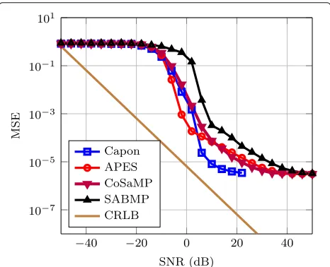
We discuss the simulation results for the spatial formula-tion. Figures 2 and 3 shows the mean square error (MSE) performance for βk andθk, respectively. The number of
antenna elementsnTandnRis 16 and the number of
snap-shotsLis 20. This is the case whereL > nR. Both APES
and Capon algorithms require L > nR to evaluate the
correlation of the received signal. The estimation perfor-mance of βk for Capon reaches an error floor because
Capon estimates are always biased [1]. APES algorithm shows the best estimation forβkfor SNR greater than−8
dB. Both SABMP and CoSaMP algorithms do not per-form well due to high under-sampling ratio. But, SABMP has better performance than CoSaMP algorithm for βk estimation. Forθk estimation, the results in Fig. 3 show that the Capon algorithm has the best performance at SNR greater than 3 dB. In Capon algorithm, at high SNR,
Fig. 2MSE performance forβkestimation. Simulation parameters: L=20,nT=16,nR=16,N=512,θk∼U(−60◦, 60◦)but on-grid, βk=ejϕkwhereϕk∼U(0, 1)
the covariance matrix of received signals becomes close to singular causing poor estimation of θk. That is why,
the results are not plotted after 22 dB. Nevertheless, the results available in Fig. 3 will serve the purpose of com-parison. SABMP performs worse in this scenario because it requires more measurements for better sparse recovery. All four algorithms reach an error floor because the grid is finite. In [35], this phenomenon is referred to as off-grid effect.
In Figs. 4 and 5, we discuss the case whenL < nR. To
simulate this case, we choosenTandnRequal to 128 and
Lis kept to 10 only. In this case, both Capon and APES
Fig. 3MSE performance forθkestimation. Simulation parameters: L=20,nT=16,nR=16,N=512,θk∼U(−60◦, 60◦)but falling
Fig. 4MSE performance forβkestimation. Simulation parameters: L=10,nT=128,nR=128,N=512,θk∼U(−60◦, 60◦)but on-grid, βk=ejϕkwhereϕk∼U(0, 1). No recovery for Capon and APES
methods
will fail to recover the estimates due to rank deficiency of received signal covariance matrix. However, CoSaMP and SABMP algorithms will still be able to work for both
βk and θk estimation. For βk estimation, SABMP
algo-rithm has better estimation than CoSaMP algoalgo-rithm up to SNR 22 dB. At high SNR, both CoSaMP and SABMP algorithms almost have the same performance for βk
estimation. Both CoSaMP and SABMP are not able to achieve the CRLB due to high under-sampling ratio. The results obtained in Fig. 5 show that SABMP algorithm has
Fig. 5MSE performance forθkestimation. Simulation parameters: L=10,nT=128,nR=128,N=512,θk∼U(−60◦, 60◦)but falling
off-grid,βk=ejϕkwhereϕk∼U(0, 1). No recovery for Capon and
APES methods
slightly better performance than CoSaMP algorithm forθk
estimation.
We show the complexity comparison in Fig. 6. The plot is shown for processing time againstnR. For all cases of
nR, the number of snapshots L is 10 for CS. For both
Capon and APES algorithms, if we keepL = 10, it will not recover the unknown parameters. However, the com-parison remains fair if we assume L at least equal to nR because the computational burden is on the
inver-sion of the covariance matrix. It can be seen that as nR increases, the processing time for Capon and APES
algorithm increases significantly. Since the size of the covariance matrix is equal tonR×nR, the size of
covari-ance matrix increases with nR. Both Capon and APES
need to invert the covariance matrix obtained from the received samples which increase the processing time with increasednR. For SABMP, the increase in computation is
mainly dependent onLin spatial formulation and is less dependent on nR. That is why SABMP complexity does
not change drastically withnR. From Fig. 6, we can note
that for nR greater than or equal to 32, the complexity
of SABMP algorithm is lower than APES but higher than Capon algorithm. CoSaMP algorithm has lower complex-ity than SABMP algorithm but is increasing significantly withnRbecause its complexity is dependent on both the
number of measurementsnR and the number of blocks
L. Since it has lower complexity, a trade-off between per-formance and complexity exists between SABMP and CoSaMP with spatial formulation.
5.2 CS temporal formulation
In this subsection, we present simulation results for the temporal formulation as an alternative to the spatial one. First, we make a comparison of resolution. Figure 7 shows
Fig. 6Complexity comparison. Simulation parameters:nT=nR, SNR
Fig. 7Resolution comparison. Simulation parameters:L=256,nT=10,
nR=10, SNR=0 dB (left), SNR=25 dB (right)
a comparison of resolution of the three algorithms. APES has wider resolution than both Capon and SABMP algo-rithms. Capon has finer resolution, but its amplitude is biased downwards. SABMP algorithm gives the best resolution because on-grid CS algorithms are based on recovery of non-zero entries. That is why SABMP algo-rithm provides a single sample at the target location. A similar behavior can be anticipated for CoSaMP algorithm because it is also an on-grid CS algorithm.
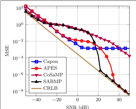
The MSE ofβkandθkestimates is shown in Figs. 8 and
9, respectively. The number of snapshotsL=256 and the array size is kept small, i.e.nT =10 andnR=10. We plot
the MSE obtained by existing algorithms Capon, APES and CoSaMP along with SABMP for comparison. CRLB is also plotted for comparison. In Fig. 8, we assume that the target lies on the grid to plot MSE ofβk and to compare
it with CRLB for knownθk. Otherwise, we need infinite
grid points to compare the performance of algorithms
Fig. 8MSE performance forβkestimation. Simulation parameters: L=256,nT=10,nR=10,N=512,θk∼U(−60◦, 60◦)but on-grid, βk=ejϕkwhereϕk∼U(0, 1)
Fig. 9MSE performance forθkestimation. Simulation parameters: L=256,nT=10,nR=10,N=512,θk∼U(−60◦, 60◦)but falling
off-grid,βk=ejϕkwhereϕk∼U(0, 1)
with CRLB. The simulation results show that SABMP per-forms better than all three Capon, APES and CoSaMP algorithms to estimate βk at high SNR. This better
per-formance of SABMP is due to its Bayesian approach and its robustness to noise. Moreover, the coherence of the sensing matrix is also less than 1 which guarantees sparse recovery at low noise. In Fig. 9, we simulate the algorithms by generatingθk anywhere randomly and not necessarily
on the grid. Due to this reason, it can be seen that MSE of
θkreached the error floor which is due to the discretized
grid and depends on the difference between the two con-secutive grid points. Forθkestimation, SABMP performs
better than APES algorithm after 10 dB but worse than Capon algorithm. CoSaMP algorithm has the worst per-formance because it cannot work well with structured sensing matrices.
The above mentioned simulation results are obtained forL > nR. Now, we discuss the case whenL < nRand
the number of snapshots is low. In the simulation results shown in Figs. 10 and 11, the number of snapshotsLis 8 only. In this case, there will be no recovery by both Capon and APES methods due to rank deficiency of covariance matrix. But both CS algorithms can work in this scenario. SABMP performs better than CoSaMP algorithm for both
βk andθk estimation. SABMP cannot achieve the CRLB
because of very low number of measurements in this case. Next, we compare the performance of algorithms at two different target locations. We choose one location at 5◦and a second location at 70◦. The simulation results in Figs. 12 and 13 show estimation performance for θk andβk respectively. The performance of all algorithms is degraded forθk = 70◦case because it comes in the low
Fig. 10MSE performance forβkestimation. Simulation parameters: L=8,nT=10,nR=10,N=512,θk∼U(−60◦, 60◦)but on-grid, βk=ejϕkwhereϕk∼U(0, 1). No recovery for Capon and APES
methods
theθk =5◦, the APES and SABMP algorithms achieve the
bound earlier thanθk=70◦.
We compare the complexity of the discussed algorithms. Figure 14 gives the processing time plotted against the number of grid pointsN. The results show that SABMP algorithm has the higher complexity than Capon and APES algorithms but lower than CoSaMP algorithm. CoSaMP algorithm has the highest complexity due to a Kronecker product involved in the construction of its sensing matrix. The complexity of SABMP is depen-dent on the number of multiple-measurement-vectors. In
Fig. 11MSE performance forθkestimation. Simulation parameters: L=8,nT=10,nR=10,N=512,θk∼U(−60◦, 60◦)but falling
off-grid,βk=ejϕkwhereϕk∼U(0, 1). No recovery for Capon and
APES methods
Fig. 12MSE performance forβkestimation. Simulation parameters: L=256,nT=10,nR=10,N=512,θk=5◦(solidlines) &θk=70◦
(dashedlines) but on-grid,βk=ejϕkwhereϕk∼U(0, 1)and is same
for all iterations
this case the number of multiple-measurement-vectors is equal to number of receive antennas. Therefore, there exists a tradeoff between performance and complexity of Capon, APES, CoSaMP and SABMP algorithm.
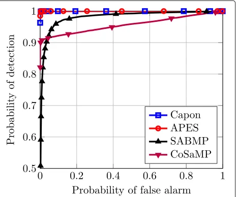
Lastly, we show a comparison of receiver operating char-acteristic (ROC) curves. At high SNR, the probability of detection for all algorithms is 1 almost for all probabilities of false alarm. Therefore, MSE criteria is better to com-pare performance of different algorithms at high SNRs. However, we can choose small SNR value of -12 dB to plot ROCs for all four algorithms. Figure 15 shows the ROC
Fig. 13MSE performance forθkestimation. Simulation parameters: L=256,nT=10,nR=10,N=512,θk=5◦(solidlines) &θk=70◦
(dashedlines) but falling off-grid,βk=ejϕkwhereϕk∼U(0, 1)and is
Fig. 14Complexity comparison. Simulation parameters:L=256 ,nT=10,nR=10, SNR=20 dB,θk∼U(−60◦, 60◦)but on-grid, βk=ejϕkwhereϕk∼U(0, 1)
comparison of the four algorithms discussed. The proba-bility of detection is close to one for both Capon and APES algorithms for a wide range of probability of false alarm. SABMP algorithm has a little worse performance than both Capon and APES algorithms because we have cho-sen a low SNR value of -12 dB but SABMP performance gains are at usually at high SNRs. CoSaMP algorithm has slightly better performance than SABMP algorithm for low values of probability of false alarm but its performance deteriorates afterwards.
Fig. 15ROC comparison. Simulation parameters:nT=10,nR=10,
SNR= −12 dB,θk∼U(−60◦, 60◦)but on-grid,βk=ejϕkwhere ϕk∼U(0, 1). (Markersare added in this plot only for the purpose of identification of different curves)
6 Conclusions
In this work, the authors solved the MIMO radar param-eter estimation problem by two methods: the spatial method for large arrays and temporal method for small arrays by a fast and robust CS algorithm. It is shown that SABMP provides the best estimates for parameter estima-tion at high SNR even when the number of targets and noise variance are unknown.
Acknowledgements
This research was funded by a grant from the office of competitive research funding (OCRF) at the King Abdullah University of Science and Technology (KAUST).
The work was also supported by the Deanship of Scientific Research (DSR) at King Fahd University of Petroleum and Minerals (KFUPM), Dhahran, Saudi Arabia, through project number KAUST-002.
The authors acknowledge the Information Technology Center at King Fahd University of Petroleum and Minerals (KFUPM) for providing high performance computing resources that have contributed to the research results reported within this paper.
Authors’ contributions
HA, SA, and TYA contributed to the formulation of the problem. HA and SA carried out the simulations. MSS and MSA commented and criticized the work to improve the manuscript. All authors read and approved the final manuscript.
Competing interests
The authors declare that they have no competing interests.
Author details
1Electrical Engineering Department, KFUPM, Dhahran, Saudi Arabia. 2Computer, Electrical and Mathematical Science and Engineering (CEMSE)
Division, KAUST, Thuwal, Saudi Arabia.
Received: 17 June 2016 Accepted: 14 December 2016
References
1. J Li, P Stoica,MIMO Radar signal processing. (John Wiley & Sons, New Jersey, 2009)
2. JA Scheer, WA Holm,Principles of modern radar: advanced techniques. (SciTech Publishing, Edison, NJ, USA, 2013)
3. DL Donoho, Compressed sensing. IEEE Trans. Inf. Theory.52(4), 1289–1306 (2006)
4. EJ Candes, PA Randall, Highly robust error correction by convex programming. IEEE Trans. Inf. Theory.54(7), 2829–2840 (2008) 5. YC Pati, R Rezaiifar, PS Krishnaprasad, inProc. 27th Asilomar Conf. Signals,
Syst. Comput. Orthogonal matching pursuit: recursive function approximation with applications to wavelet decomposition (IEEE, 1993), pp. 40–44
6. D Needell, R Vershynin, Uniform uncertainty principle and signal recovery via regularized orthogonal matching pursuit. Found. Comput. Math.9(3), 317–334 (2008)
7. DL Donoho, Y Tsaig, I Drori, J-L Starck, Sparse solution of underdetermined systems of linear equations by stagewise orthogonal matching pursuit. IEEE Trans. Inf. Theory.58(2), 1094–1121 (2012)
8. D Needell, JA Tropp, CoSaMP: Iterative signal recovery from incomplete and inaccurate samples. Appl. Comput. Harmon. Anal.26(3), 301–321 (2009)
9. ME Tipping, Sparse Bayesian learning and the relevance vector machine. J. Mach. Learn. Res.1, 211–244 (2001)
10. S Ji, Y Xue, L Carin, Bayesian compressive sensing. IEEE Trans. Signal Process.56(6), 2346–2356 (2008)
11. P Schniter, LC Potter, J Ziniel, in2008 Inf. Theory Appl. Work. Fast Bayesian matching pursuit (IEEE, 2008), pp. 326–333
12. AA Quadeer, TY Al-Naffouri, Structure-based Bayesian sparse reconstruction. IEEE Trans. Signal Process.60(12), 6354–6367 (2012) 13. M Masood, TY Al-Naffouri, Sparse reconstruction using distribution
14. JHG Ender, On compressive sensing applied to radar. Signal Process.
90(5), 1402–1414 (2010)
15. Y Yu, AP Petropulu, HV Poor, MIMO radar using compressive sampling. IEEE J. Sel. Top. Signal Process.4(1), 146–163 (2010)
16. P Stoica, P Babu, J Li, SPICE: A sparse covariance-based estimation method for array processing. IEEE Trans. Signal Process.59(2), 629–638 (2011) 17. M Rossi, AM Haimovich, YC Eldar, Spatial compressive sensing for MIMO
radar. IEEE Trans. Signal Process.62(2), 419–430 (2014)
18. Y Yu, S Sun, RN Madan, A Petropulu, Power allocation and waveform design for the compressive sensing based MIMO radar. IEEE Trans. Aerosp. Electron. Syst.50(2), 898–909 (2014)
19. Z Yang, L Xie, C Zhang, Off-grid direction of arrival estimation using sparse Bayesian inference. IEEE Trans. Signal Process.61(1), 38–43 (2013) 20. T Huang, Y Liu, H Meng, X Wang, Adaptive matching pursuit with
constrained total least squares. EURASIP J. Adv. Signal Process.2012(1), 252 (2012)
21. S Jardak, S Ahmed, M-S Alouini, in2015 Sens. Signal Process. Def. Low complexity parameter estimation for off-the-grid targets (IEEE, 2015) 22. S Jardak, S Ahmed, M-S Alouini, in2014 Int. Radar Conf. Low complexity
joint estimation of reflection coefficient, spatial location, and Doppler shift for MIMO-radar by exploiting 2D-FFT (IEEE, 2014)
23. KV Mishra, M Cho, A Kruger, W Xu, Spectral super-resolution with prior knowledge. IEEE Trans. Signal Process.63(20), 5342–5357 (2015) 24. Candè,s, JK Romberg, T Tao, Stable signal recovery from incomplete
and inaccurate measurements. Commun. Pure Appl. Math.59(8), 1207–1223 (2006)
25. J Li, P Stoica, MIMO radar with colocated antennas. IEEE Signal Process. Mag.24(5), 106–114 (2007)
26. H Jiang, J-K Zhang, KM Wong, Joint DOD and DOA estimation for bistatic MIMO radar in unknown correlated noise. IEEE Trans. Veh. Technol.
64(11), 5113–5125 (2015)
27. P Stoica, Target detection and parameter estimation for MIMO radar systems. IEEE Trans. Aerosp. Electron. Syst.44(3), 927–939 (2008) 28. EJ Candes, T Tao, Decoding by linear programming. IEEE Trans. Inf.
Theory.51(12), 4203–4215 (2005)
29. N Yu, Y Li, Deterministic construction of Fourier-based compressed sensing matrices using an almost difference set. EURASIP J. Adv. Signal Process.2013(1), 155 (2013)
30. H Ali, S Ahmed, TY Al-Naffouri, M-S Alouini, inInt. Radar Conf. Reduction of snapshots for MIMO radar detection by block/group orthogonal matching pursuit (IEEE, 2014)
31. M Masood, TY Al-Naffouri, inIEEE Int. Conf. Acoust. Speech Signal Process. Support agnostic Bayesian matching pursuit for block sparse signals (IEEE, 2013), pp. 4643–4647
32. DL Donoho, M Elad, Optimally sparse representation in general (nonorthogonal) dictionaries via1minimization. Proc. Natl. Acad. Sci. 100(5), 2197–2202 (2003)
33. R Gribonval, M Nielsen, Sparse representations in unions of bases. IEEE Trans. Inf. Theory.49(12), 3320–3325 (2003)
34. RG Baraniuk, V Cevher, MF Duarte, C Hegde, Model-based compressive sensing. IEEE Trans. Inf. Theory.56(4), 1982–2001 (2010)
35. S Fortunati, R Grasso, F Gini, MS Greco, K LePage, Single-snapshot DOA estimation by using compressed sensing. EURASIP J. Adv. Signal Process.
2014(1), 120 (2014)
Submit your manuscript to a
journal and benefi t from:
7Convenient online submission
7Rigorous peer review
7Immediate publication on acceptance
7Open access: articles freely available online
7High visibility within the fi eld
7Retaining the copyright to your article