www.biogeosciences.net/3/571/2006/ © Author(s) 2006. This work is licensed under a Creative Commons License.
Biogeosciences
Towards a standardized processing of Net Ecosystem Exchange
measured with eddy covariance technique: algorithms and
uncertainty estimation
D. Papale1, M. Reichstein2, M. Aubinet3, E. Canfora1, C. Bernhofer4, W. Kutsch2, B. Longdoz5, S. Rambal6, R. Valentini1, T. Vesala7, and D. Yakir8
1Department of Forest Science and Environment, University of Tuscia, 01100 Viterbo, Italy 2Max-Planck Institut fur Biogeochemie, P.O. Box 100164, 07701 Jena, Germany
3Facult´e des Sciences Agronomiques, Avenue de la Facult´e d’Agronomie 8, 5030 Gembloux, Belgium
4Dept. of Meteorology, Institute of Hydrology and-Meteorology, Technische Universitat Dresden, 01062 Dresden, Germany 5Ecologie et Ecophysiologie Foresti`eres, Centre de Nancy, 54280 Champenoux, France
6Dream CEFE-CNRS, 1919 route de Mende, 34293 Montpellier, France
7Department of Physical Sciences, University of Helsinki, P.O. Box 64, FIN-00014, Finland
8Dept. of Environmental Sciences and Energy Research, Weizmann Institute of Science, P.O. Box 26, 76100 Rehovot, Israel
Received: 7 June 2006 – Published in Biogeosciences Discuss.: 13 July 2006
Revised: 26 October 2006 – Accepted: 16 November 2006 – Published: 27 November 2006
Abstract. Eddy covariance technique to measure CO2,
wa-ter and energy fluxes between biosphere and atmosphere is widely spread and used in various regional networks. Cur-rently more than 250 eddy covariance sites are active around the world measuring carbon exchange at high temporal res-olution for different biomes and climatic conditions. In this paper a new standardized set of corrections is introduced and the uncertainties associated with these corrections are as-sessed for eight different forest sites in Europe with a total of 12 yearly datasets. The uncertainties introduced on the two components GPP (Gross Primary Production) and TER (Terrestrial Ecosystem Respiration) are also discussed and a quantitative analysis presented. Through a factorial analy-sis we find that generally, uncertainties by different correc-tions are additive without interaccorrec-tions and that the heuristic u∗-correction introduces the largest uncertainty. The results
show that a standardized data processing is needed for an ef-fective comparison across biomes and for underpinning inter-annual variability. The methodology presented in this paper has also been integrated in the European database of the eddy covariance measurements.
Correspondence to: D. Papale ([email protected])
1 Introduction
The eddy covariance technique provides unique measure-ments of CO2, water and energy fluxes between the
bio-sphere and the atmobio-sphere at the ecosystem scale. Currently, more than 250 eddy covariance towers are acquiring data around the world (Baldocchi et al., 2001), covering different climate conditions, land use and land cover changes, some of them running continuously for more than 10 years. The eddy covariance technique is based on high frequency (10-20 Hz) measurements of wind speed and direction as well as CO2and H2O concentrations at a point over the canopy using
a three-axis sonic anemometer and a fast response infrared gas analyzer (Aubinet et al., 2000; Aubinet et al., 2003a). Assuming perfect turbulent mixing these measurements are typically integrated over periods of half an hour (Goulden et al., 1996) building the basis to calculate carbon and water balances from daily to annual time scales.
Varying footprints can be a source of errors and uncertain-ties that can affect the data quality, particularly if the ecosys-tem is inhomogeneous and patchy (G¨ockede et al., 2006). In addition, several errors due to instrumentation limits may ap-pear (acquisition frequency, sensor separation, fluctuation at-tenuation in closed systems, etc. . . ). Most of these problems can be solved by applying correction procedures accordingly. However, it was shown by different authors (Aubinet et al., 2000; Goulden et al., 1996; Gu et al., 2005), independently of the preceding problems, eddy flux measurements can un-derestimate the net ecosystem exchange during periods with low turbulence and thus limited air mixing. This underes-timation acts as a selective systematic error: it only occurs during the night when there is a net emission of CO2by the
ecosystem. As a consequence, the ecosystem respiration is underestimated and the carbon sequestration overestimated (Moncrieff et al., 1996).
Massman and Lee (2002) listed the possible causes of the night-time flux error. There is now a large consensus to recognise that the most probable cause of error is the presence of small scale movements associated with drainage flows or land breezes that take place in low turbulence con-ditions and create a decoupling between the soil surface and the canopy top. In these conditions, advection becomes an important term in the flux balance and cannot be neglected anymore. It was recently suggested (Finnigan et al., 2006) that, contrary to what was thought before, advection proba-bly affects most of the sites, including almost flat and homo-geneous ones. Direct advection flux measurements are diffi-cult to measure as they require several measurement towers at the same site. Attempts were made notably by Aubinet et al. (2003b), Feigenwinter et al. (2004), Staebler and Fitz-jarrald (2004) and Marcolla et al. (2005). They found that advection fluxes were usually significant during calm nights. However, in most cases, the measurement uncertainty was too large to allow their precise estimation. In addition, such direct measurements require a too complicated set up to al-low routine measurements at each site.
In practice, the night flux problem is by-passed by discard-ing the data corresponddiscard-ing to low mixed periods and replac-ing them by an assessment based either on the parameterisa-tion of the night flux response to the climate or on look up tables (Falge et al., 2001; Papale and Valentini, 2003; Reich-stein et al., 2005). The friction velocity is currently used as a criterion to discriminate low and well mixed periods. This approach is generally known as the “u∗correction”.
Although being currently the best and most widely used method to circumvent the problem, the u∗ correction is
af-fected by several drawbacks and must be applied with care. First, an implicit application of the correction could lead to even bigger errors: indeed, during calm night conditions, the CO2can be either removed by advection or stored in the
canopy air. In the first case, the application of a u∗
correc-tion is fully justified. However, in the second case, the CO2
stored in the canopy air would be removed by the turbulence
as soon as it restarts. It would be captured at this moment by the eddy covariance system. If a u∗ correction had been
applied during the storage period, this flux would thus have been counted twice. One way to avoid this problem is to first correct the data for storage and then apply the u∗selection.
However, this requires reliable CO2 storage measurements
which are not always available at all sites. The best way to compute storage flux is to deduce it from CO2concentration
profiles made in the canopy. However, at many sites, a dis-crete estimation based only on the concentration at the tower top is used. It is likely that, in tall forests sites, such estima-tion is insufficient as it does not take the large concentraestima-tion increase in the lower air layers into account. It is therefore important to understand the potential errors introduced using the discrete approach instead of the profile system.
Another problem with the u∗correction is that it depends
on the operator’s subjectivity. Indeed, the u∗threshold used
to discriminate well and poorly mixed data is generally cho-sen by visual inspection. Different alternative heuristic meth-ods were proposed to automatically determine the appropri-ate u∗ threshold value (Gu et al., 2005; Reichstein et al.,
2003; Reichstein et al., 2005).
Finally, the hypotheses underlying the u∗ correction are
still debatable: firstly it is based on the assumption that flux in calm conditions can be inferred from measurements made in windy conditions, which is not proven. Secondly, it sup-poses that measurements made during turbulent periods are free of errors which is questioned by recent experiment re-sults (Cook et al., 2004; Lee et al., 2004; Wohlfahrt et al., 2005).
There is a high heterogeneity in terms of quality and meth-ods used in data processing. Many improvements in the Eddy measurements treatments were presented and applied over the last 10 years, often detailed information about the data processing methods were not available and important vari-ables like the CO2storage under the canopy were not
mea-sured. For this reason it is very important to have a set of tools to process all the datasets available with a standardized method with the aim to improve their quality, particularly if the data are used for interannual analysis or site intercompar-isons, and where raw data are not available and for this rea-son it is impossible to use others criteria recently proposed (Rebmann et al., 2005; Ruppert et al., 2006).
It is also crucial to assess the effect of these integral flux corrections on data and the errors and uncertainties intro-duced. The sequence of analyses presented in this paper is based solely on half-hourly flux data to find the cases affected by common problems like spikes or low turbulence. Method-ological uncertainties introduced by the different quality con-trol procedures (e.g. u∗ threshold selection) are
Table 1. Sites and years used and main characteristics. MF=mixed forest, ENF=evergreen needle forest, EBF=evergreen broadleaves
forest, DBF=deciduous broadleaves forest, ECO=Ecosystem type, MAT=Mean Annual Temperature (◦C), Prec=Annual precipitation (mm),
LAI=Leaf Area Index (maximum).
Code Years Name Lat. Long. ECO MAT Prec LAI Topography Reference
BE01 2001 Vielsalm 50◦180N 5◦590E MF 7.5 1000 5.1 Slope 3% (Aubinet et al., 2001)
DE02 2001, 2002 Tharandt 50◦570N 13◦340E ENF 7.7 820 7.6 Gently sloped (Bernhofer et al., 2003)
DE03 2001, 2002 Hainich 51◦040N 10◦270E DBF 6.8 775 6.4 Gently sloped (Knohl et al., 2003)
FI01 2001, 2002 Hyyti¨al¨a 61◦500N 24◦170E ENF 3.8 709 6.7 Flat (Suni et al., 2003)
FR01 2001, 2002 Hesse 48◦400N 07◦030E DBF 9.9 975 7.65 Slope 3% (Granier et al., 2000)
FR04 2002 Puechabon 43◦440N 03◦350E EBF 13.5 872 2.9 Flat (Rambal et al., 2004)
IL01 2002 Yatir 31◦200N 35◦030E ENF 18.2 280 2 Undulated (Grunzweig et al., 2003)
IT03 2002 Roccarespampani 42◦240N 11◦550E DBF 15.2 876 1.4 Flat/Gently sloped (Tedeschi et al., 2006)
2 Materials and methods
2.1 Sites and processing overview
For the present analyses, 12 annual datasets of CO2exchange
have been used from eight European eddy covariance sites (Table 1). The data were first storage corrected, then a spike detection technique was applied and, after that, filtered for low turbulence conditions (low u∗). After these checks the
yearly datasets were gap filled and the two components Gross Primary Production (GPP) and Terrestrial Ecosystem Respi-ration (TER) were estimated.
The storage flux (Sc) is calculated as (Aubinet et al.,
2001):
Sc= Pa R·Ta
Z h
0
∂c (z) ∂t dz
where Pa is the atmospheric pressure,Ta is the air
temper-ature,R is the molar gas constant,cis the CO2
concentra-tion measured along a vertical profile,his the profile height. In practice the derivatives are approximated by finite differ-ences between two successive measurements and the inte-grals are approximated by weighted sums of the concentra-tions measured at the different profile levels (generally be-tween 4 and 7 measurement points). There are however sites where the profile system is not present or where it was not available during the first years of activity (FR01, FR04, IL01, IT03 in this paper). For these sites the only way to assess the storage flux is using the discrete approach, where the CO2
concentration measured at the top of the tower is considered constant inside the canopy.
2.2 The spike detection method
Eddy covariance measurements are often affected by spikes, due to different reasons both bio-physical (changes in the footprint or fast changes in turbulence conditions) and instru-mental (e.g. water drops on sonic anemometer or on open path IRGA). The spikes affecting the single instantaneous measurement (high frequency spikes) are removed before
the half-hourly average flux is calculated. However, spikes could also occur in the time series of the half hourly flux values and an outlier detection technique was applied to find these occasional spikes in the half-hourly flux data. These spikes commonly do not affect directly the annual NEE but can affect the quality of the gapfilled datasets. The algo-rithm used to detect the spikes is based on the position of each half hourly value with respect to the values just before and after and it is applied to blocks of 13 days and sepa-rately for daytime and night-time data. These night-time and daytime periods have been extended adding one value form the other period at the borders, needed to calculate di (see
later); night-time data were selected according to a global ra-diation threshold of 20 Wm−2, cross-checked against sunrise and sunset data derived from the local time and standard sun-geometrical routines. The outlier detection was based on the double-differenced time series, using the median of absolute deviation about the median (MAD) that is a robust outlier estimator (Sachs, 1996).
For each NEEi half hourly data thed value is calculated
as:
di =(NEEi−NEEi−1)−(NEEi+1−NEEi) (1)
and the value is flagged as spike if:
di < Md−
z·MAD
0.6745
(2) or
di > Md+
z·MAD
0.6745
(3) where Md is the median of the differences, MAD is defined as
MAD=median(|di−Md|) (4)
andzis a threshold value.
u* threshold
0.05 0.10 0.15 0.20 0.25 0.30 0.35 0.40 0.45 0.50
Percentage
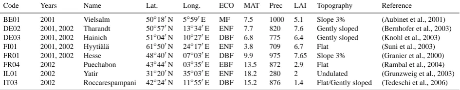
[image:4.595.51.281.77.255.2]0 5 10 15 20 25 30
Fig. 1. Example of the variability in the u∗ threshold found with
the bootstrapping. Lines indicate mean (yellow), median (red), 5% (green) and 95% (blue) values. BE01 01, storage with discrete
ap-proach, spikes thresholdz= 5.5.
2.3 The u∗threshold selection and uncertainty
The u∗-threshold was specifically derived for each site using
a 99% threshold criterion on night-time data as described by (Reichstein et al., 2005). For the determination of the u∗
-threshold, the data set is split into six temperature classes of equal sample size (according to quantiles) and for each temperature class, the set is split into 20 equally sized u∗
-classes. The threshold is defined as the u∗-class where the
average night-time flux reaches more than 99% of the aver-age flux at the higher u∗-classes. The threshold is only
ac-cepted if for the temperature class, temperature and u∗ are
not or only weakly correlated (|r|<0.4) The final threshold is defined as the median of the thresholds of the (up to) six temperature classes. This procedure is applied to the subsets of four 3-month periods (January–March, April–June, July– September and October–December) to account for seasonal variation of vegetation structure.
The u∗-threshold is reported for each period, but the whole
data set is filtered according to the highest threshold found (conservative approach). In cases where no u∗-threshold
could be found in any of the 3-month periods with this ap-proach, it is set to the 90% percentile of the data (i.e. a min-imum 10% of the data are retained). A minmin-imum threshold is set to 0.1 ms−1for forest canopies and 0.01 ms−1for short vegetation sites that commonly have lower u∗values (Falge
et al., 2001; Gu et al., 2005). To be more conservative, in ad-dition to the data acquired when u∗was below the threshold,
the first half hour measured with good turbulence conditions after a period with low turbulence is also removed.
This procedure is repeated 100 times within a bootstrap-ping technique to asses the uncertainty of the u∗ threshold
detection, where the whole annual dataset is bootstrapped (Efron and Tibshirani, 1993). The bootstrapping was car-ried in the following way: in each bootstrapping step, the whole year was sampled on a half-hourly basis into a data set with 17 520 data points, where each half-hour can be drawn several times. Theoretically this procedure could lead to the case that considerably less points from a particular season (or from particular meteorological situations) are drawn in-troducing additional uncertainty. However due to the large number of data points (17 520 half-hourly values) this is very unlikely. For example the probability that less than 4000 points are drawn from summer is 1.14×10⁻¹¹. The advan-tage of the bootstrapping is that parameters can be estimated without assumptions about the normal distribution and using also small samples size The effect of missing data is also in-cluded since missing data points are sampled with the same probability. The 5% and 95% percentiles of the 100 boot-strapped threshold estimates are taken as confidence interval boundaries (Fig. 1).
2.4 Gap filling and partitioning of carbon fluxes
To compare the effect of the different checks and filters ap-plied at different time resolution (from daily to annual), all the datasets had to be filled. We used as gap-filling technique the method described in Reichstein et al. (2005) that exploits both the co-variation of fluxes with meteorological variables and the temporal autocorrelation of fluxes. The potential ef-fect of different gap-filling methods on annual NEE is out of the scope of this paper, but it is systematically addressed in an ongoing work by Moffat et al. (2006)1and seems to be generally small for the methods investigated (Papale et al., 2006).
The partitioning between Gross Primary Production and Terrestrial Ecosystem Respiration has been done according to the method proposed in Reichstein et al. (2005).
3 Results and discussion
3.1 Variability and uncertainty of u∗threshold values
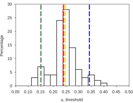
For the 12 annual datasets used in this analysis, the different u∗ thresholds and the 5% and 95% percentiles obtained
af-ter storage correction and spike detection are in a range that varies between 0.1 and 0.7 m s−1, as reported in Fig. 2. Note-worthy, the u∗ threshold can be different for different sites,
from very low values and low uncertainty as in FR01 to high values and uncertainty as in DE03, but is generally between 0.15 and 0.25 m s−1. This variability could be related to the characteristic of the site like canopy structure that have an
1Moffat, A., Papale, D., Reichstein, M., et al.: Comprehensive
effect on the capacity of the eddies to penetrate in the for-est, and topography that is one of the factors responsible for advection. In FI01 the threshold changes quite strongly be-tween one year and the other and this could be related to one thinning of the forest that has been done in winter 2002. To better understand this variability in the u∗threshold
be-tween sites more detailed analysis are necessary and impor-tant information could come from the advection studies and experiments that are currently carried out (Feigenwinter et al., 2006). In any case the bootstrapping method provides a non-parametric estimate of the u∗-threshold uncertainty that
is otherwise only hard to obtain. It is thus recommended to include an uncertainty estimate of the u∗-threshold via a
bootstrapping or similar sampling technique, which repre-sents an important improvement over methods just providing a point estimate (Gu et al., 2005).
The u∗-threshold value and his uncertainty given by the
difference between the 5 and 95 percentiles must however not be confounded with the uncertainty introduced in the flux data (e.g. annual sums) as will be shown later in the paper (Fig. 9 later in this paper).
This method for the u∗-threshold selection has been
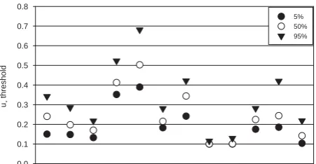
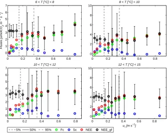
ap-plied in this study only to forest sites, however the use of the maximum value found in the four 3-month periods makes this method also appropriate for ecosystems where the veg-etation structure change more rapidly like agricultural and managed grassland ecosystems. Figure 3 shows the effect of the different corrections and in particular u∗filtering to the
fluxes. The plots are relative to BE01 with storage calculated using discrete approach and each of the 4 subplots is obtained using April to September night-time data in the same range of temperatures (indicated in the title of the subplot). The temperature ranges are automatically chosen in a way that the same number of data are used in each subplot. Also the 12 u∗classes for each temperature class are automatically
se-lected to have the same number of data in each classes. If u∗
correction would not be needed NEE should be independent from u∗. The differences between NEE gf and NEE in the u∗
classes above the threshold are due to the spike filtering but over all to the first measurement with high u∗after a period
with low turbulence that are also removed as explained be-fore in the text. It is possible to see that Fc decrease with low turbulence conditions but the storage flux doesn’t compen-sate it while after the corrections the night time fluxes are, in average, more independent from u∗as expected.
3.2 Effect of storage and u∗correction
According to the eddy covariance data processing method, the CO2fluxes are corrected by storage fluxes and after that
filtered by u∗ to remove measurements acquired during low
turbulence conditions. These two corrections have to be done in the order described above to avoid the double counting ef-fect, i.e. that (turbulent+storage) fluxes are removed during night with low u∗(and so the potentially high storage flux
ig-BE01 2001
DE02 2001
DE02 2002
DE03 2001
DE03 2002
FI01 2001
FI01 2002
FR01 2001
FR01 2002
FR04 2002
IL01 2002
IT03 2002
u*
threshold
0.0 0.1 0.2 0.3 0.4 0.5 0.6 0.7 0.8
[image:5.595.312.538.68.185.2]5% 50% 95%
Fig. 2. Median and selected percentiles of the u∗threshold
distri-bution determined by the bootstapping for the 12 yearly datasets for
discrete approach storage calculation and spike thresholdz= 5.5.
nored) while during the following morning the depletion of the storage is accounted for (Aubinet et al., 2002). Figure 4 shows the annual NEE obtained for the different sites/years by using different treatments: the recommended one (first storage, then u∗), u∗correction only, storage correction only,
and no corrections. The little differences between data with-out corrections and data only storage corrected, that theoret-ically should be exactly the same for the annual NEE, are due to the different number of gaps (e.g. if storage flux is missing, but not turbulent flux). It is possible to see that the differences between the four annual NEE presented for each site and year vary a lot from site to site. For example for FR01 the differences are in the order of 30–40 gC m−2yr−1 (between 5 and 10%) while for IT03 the differences are very strong and the site changes from sink to source of carbon using the different thresholds. The effect of the u∗filtering
leads to reductions of the annual NEE as expected except for FR01 where the changes are in the opposite direction. This could be due to the small u∗-threshold value used for this site
that have a limited impact on the annual NEE. Another inter-esting point is that the double counting problem (differences between right correction and only u∗)is evident for most of
the sites (BE01, DE02, FR04, IL01 and IT03) while for some sites it is not clear: in FI01 there is not a clear difference and this can be due to the small effect that the u∗ filtering have
on the annual NEE (see later Fig. 8 and Fig. 9a), the same happens in FR01 where the trend changes from one year to the other and can be also related to the little impact of the u∗
filtering as discussed before. In DE03 the trend is in the op-posite direction as expected and could be related to the pres-ence of strong horizontal advection where u∗filtering could
0 0.2 0.4 0.6 0.8 0
1 2 3 4 5 6 7
Fluxes [umolCO
2
m
−2
s
−1
]
6 < T [°C] < 8
0 0.2 0.4 0.6 0.8
0 2 4 6 8 10
8 < T [°C] < 10
0 0.2 0.4 0.6 0.8
0 1 2 3 4 5 6 7
10 < T [°C] < 12
0 0.2 0.4 0.6 0.8
0 2 4 6 8 10
12 < T [°C] < 15
u* [m s−1]
[image:6.595.132.468.64.329.2]5% 50% 95% Fc Sc NEE NEE_gf
Fig. 3. Effect of the different corrections on the relation between u∗ and fluxes (BE01 01). Data used in these plots are from April
to September, night time only. Each subplot is obtained using data acquired when air temperatures was similar so that the fluxes (only respiration) are expected to be independent from turbulence. The grey lines are the selected u* threshold and the 5% and 95% percentiles of the 100 bootstapped threshold estimates. NEE gf is the NEE after all the filtering and gapfilling and the errors bars indicate the standard
deviation of NEE in each u∗class. The method used to create these plots is conceptually similar to the method use to find the u∗threshold
but it is based on 6 months period and different temperature classes.
gC m
-2 yr
-1
-800 -700 -600 -500 -400 -300 -200 -100 0 100
u* and storage
only storage only u*
no corrections
BE01 2001
DE02 2001
DE02 2002
DE03 2001
DE03 2002
FI01 2001
FI01 2002
FR01 2001
FR01 2002
FR04 2002
IL01 2002
IT03 2002
Fig. 4. Effect of storage and u∗corrections on annual NEE.
3.3 Effect of the filtering techniques used
The amount of data removed by the filtering algorithms was found variable as depicted in Table 2. The “Missing” col-umn indicates the percentage of missing NEE values (not measured or affected by evident measurement problems like pump or gas analyzer broken); columns labelled as “Spike” show the percentages of additionally removed data, due to spike detection, using the three different thresholds. The
three “u∗” columns of Table 2 show the percentages of
addi-tionally removed data because acquired under stable condi-tions (with low u∗)according with the three thresholds used.
The last column lists the percentages of data removed using a “mean” configuration with spike threshold 5.5 and 50% u∗
threshold. It is evident that the largest percentages of data is removed by the u∗filtering, while the spike removal keeps
largest part of the data untouched. Up to more than 50% of the night-time data are subject to this u∗-based filter, while
daytime data are less affected by turbulence problems, ex-cept for DE03 where in 2002 up to 50% of daytime data were filtered with the highest u∗threshold.
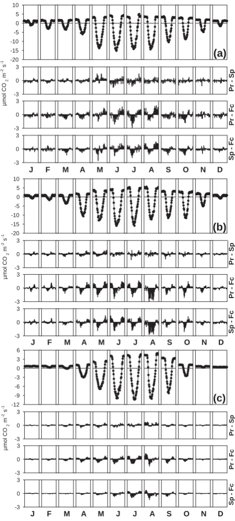
All the integral flux corrections and checks described above have an effect at different time scales, from the av-erage daily trend to the annual sums. Figure 5 shows the monthly mean diurnal NEE trends for three site/years ob-tained using three different storage correction: with the stor-age term assessed using a CO2 concentration profile in the
canopy (NEE pr), assessed using the discrete approach us-ing only the CO2 concentration measured on the top of the
[image:6.595.49.279.432.554.2]Table 2. Percentage of half hourly data (storage corrected with the best method available at each site: BE01, DE02, DE03 and FI01 profile, FR01, FR04, IL01 and IT03 discrete approach) deleted in the different conditions. Missing: data not measured or deleted due to evident
technical problems, Spike: additional data removed with the spike detection technique according with the different thresholds, u∗: additional
data removed (after previous removal of spikes using threshold 5.5) due to low u∗conditions according with the three different thresholds,
Total: the percentage of data removed summing missing data, spike withz= 5.5 and u∗50%. The two numbers in italic are the percentages
of night-time and daytime respectively for each site. All the percentages are relative to the year.
Site year Missing Spike 4 Spike 5.5 Spike 7 u∗5% u∗50% u∗95% Total
BE01 01 7.48 7.03 1.06 1.11 0.46 0.38 0.19 0.13 13.09 20.03 20.21 29.82 28.04 38.92 28.14 37.23
7.92 1.02 0.54 0.26 6.15 10.61 17.17 19.06
DE02 01 9.82 8.61 1.89 2.28 1.02 1.36 0.46 0.68 13.35 21.87 17.45 28.15 28.15 42.18 28.29 38.12
11.04 1.50 0.67 0.23 4.83 6.76 14.12 18.47
DE02 02 16.64 14.21 1.76 2.31 0.95 1.40 0.41 0.64 11.63 18.74 15.66 24.52 21.17 31.36 33.25 40.14
19.08 1.21 0.49 0.18 4.51 6.79 10.98 26.36
DE03 01 15.55 17.80 1.30 1.44 0.58 0.64 0.24 0.30 20.03 25.83 31.29 38.93 39.36 47.01 47.42 57.36
13.30 1.16 0.53 0.18 14.24 23.65 31.71 37.48
DE03 02 15.67 18.58 1.20 1.05 0.64 0.62 0.30 0.29 28.53 35.42 40.77 47.35 56.31 61.70 57.08 66.55
12.76 1.35 0.66 0.32 21.63 34.19 50.91 47.61
FI01 01 14.25 19.38 1.27 1.58 0.59 0.76 0.29 0.38 15.64 21.15 21.68 28.92 29.12 37.52 36.52 49.06
9.12 0.97 0.41 0.21 10.14 14.45 20.71 23.98
FI01 02 15.59 21.76 1.27 1.40 0.51 0.62 0.19 0.23 22.00 28.53 30.01 37.63 37.47 45.22 46.11 60.00
9.42 1.13 0.41 0.15 15.47 22.40 29.71 32.23
FR01 01 7.63 8.94 2.84 3.08 1.87 2.04 1.13 1.12 15.26 23.29 15.26 23.29 17.92 26.75 24.75 34.27
6.31 2.60 1.70 1.14 7.23 7.23 9.09 15.24
FR01 02 8.41 9.24 2.63 3.46 1.60 1.91 0.87 1.04 16.50 24.08 16.60 24.19 20.09 28.55 26.61 35.33
7.58 1.80 1.29 0.70 8.92 9.02 11.62 17.89
FR04 02 9.51 9.92 1.88 2.18 0.86 1.00 0.41 0.43 31.60 46.77 37.45 52.67 46.28 60.31 47.82 63.60
9.10 1.59 0.71 0.38 16.44 22.24 32.25 32.04
IL01 02 18.20 17.32 1.67 1.87 0.92 1.12 0.48 0.63 23.58 38.66 29.49 46.70 36.89 55.37 48.61 65.14
19.09 1.47 0.72 0.33 8.49 12.28 18.42 32.09
IT03 02 6.96 6.54 2.40 2.71 1.61 1.82 0.86 0.96 20.15 34.20 27.56 45.37 41.84 62.44 36.13 53.72
7.39 2.09 1.40 0.75 6.11 9.75 21.24 18.54
with underestimation of night-time respiration and overesti-mation of daytime carbon uptake. It is also clear that the ef-fect of the storage correction is different in the three sites, with minor effect for FI01 (Fig. 5c) that could be due to the more open canopy structure in particular in 2002 due to the thinning, but also related to the overall flux magni-tude that is less compared to the others two sites. Analyzing the differences between the two storage correction options it appears that the differences are lower with respect to the comparison between storage and no storage correction at all and also the pattern is different and less systematic but still present (e.g. BE01 June and July, DE02 April and May, FI01 May and August). This problem is quite common in the old datasets where often the profile systems were not available. To better assess the storage flux in these datasets would be in-teresting to explore the possibility to retrieve a “storage cor-rection factor” through a relation between the storage mea-sured with the profile system and a series of variables like CO2concentration at top of the tower, wind speed and
direc-tion, atmospheric pressure, temperature, etc. using methods able to find also complex relations between variables like Ar-tificial Neural Networks (Papale and Valentini, 2003).
Figure 6 shows the effect of the different thresholdszin the spike removing algorithm. The average daily trend has been calculated after filtering the data according with the 3z
values of 4, 5.5 and 7 and also without performing the spike detection at all. It is important to remark that the presence of spikes is related to different aspects and in particular to the site characteristics but also to the data screening operated by the PI. It is possible to see that the spike removing affects the mean diurnal cycles less than the storage correction. In addi-tion, there is not a clear trend also if it seems that the major part of spikes for DE03 has been detected as “respiration” spikes and that there is a relation between the flux and the spike filtering magnitudes.
The analysis of the average daily trends does not give a clear quantitative information about the effect on the daily to annual budget. We characterise the intrinsic uncertain-ties of the correction methods by the difference between the maximum flux and minimum flux obtained depending on the method for each day, week or month. These uncertainties are presented in Fig. 7 as box-plots, where for example the me-dian range of the different methods for daily fluxes across all the sites was 0.4 gC m−2day−1, considered as the me-dian uncertainty of the corrections applied. As expected, the uncertainty is bigger in the daily sums compared to 8-daily and monthly aggregations. The u∗threshold selection is the
µ
mol CO
2
m
-2 s
-1
Pr - Sp
Pr - Fc
Sp - Fc
-20 -15 -10 -5 0 5 10
-3 0 3
-3 0 3
-3 0 3
J F M A M J J A S O N D
(a)
µ
mol CO
2
m
-2 s
-1
Pr - Sp
Pr - Fc
Sp - Fc
-20 -15 -10 -5 0 5 10
-3 0 3
-3 0 3
-3 0 3
J F M A M J J A S O N D
(b)
µ
mol CO
2
m
-2 s
-1
Pr - Sp
Pr - Fc
Sp - Fc
-12 -9 -6 -3 0 3 6
-3 0 3
-3 0 3
-3 0 3
J F M A M J J A S O N D
[image:8.595.47.289.63.598.2](c)
Fig. 5. Effect of different storage measurement methods on monthly mean diurnal NEE trends for three sites: BE01 01 (a), DE02 01 (b) and FI01 02 (c). In the upper panel diurnal cycle calculated from NEE pr is shown; the other three panels the residuals respectively between the two storages (Pr–Sp), between storage from profile and no storage correction (Pr–Fc) and between storage from discrete approach and no storage correction (Sp–Fc).
µ
mol CO
2
m
-2 s
-1
z = 4.0
z = 5.5
z = 7.0
-9 -6 -3 0 3
-2 0 2
-2 0 2
-2 0 2
J F M A M J J A S O N D
(a)
µ
mol CO
2
m
-2 s
-1
z = 4.0
z = 5.5
z = 7.0
-30 -20 -10 0 10
-2 0 2
-2 0 2
-2 0 2
J F M A M J J A S O N D
(b)
µ
mol CO
2
m
-2 s
-1
z = 4.0
z = 5.5
z = 7.0
-20 -15 -10 -5 0 5 10
-2 0 2
-2 0 2
-2 0 2
J F M A M J J A S O N D
[image:8.595.311.551.63.604.2](c)
Fig. 6. Effect of different spike detection thresholdszon monthly mean diurnal NEE trends for three sites: IL01 02 (a), DE03 02 (b) and IT03 02 (c). In the upper panel diurnal cycles calculated from data before spike detection is shown; the others three panels the
residuals respectively between original andz= 7, between original
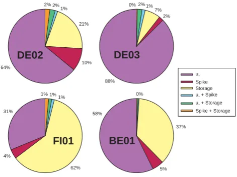
NEE an ANOVA (Analysis of variance) has been performed using the annual NEE coming from the sites where the stor-age is measured also using the profile system. The summary of the results are shown in Fig. 8. The main source of uncer-tainty is confirmed to be u∗that is the main factor for three
sites and in the fourth (FI01) is still important with 31%. In addition it has to be noted that this analysis give information about the relative role of the different corrections in the to-tal uncertainty definition but it is not directly related with the magnitude of the uncertainty. For DE03 u∗has a strong
ef-fect (88%) and this is due to the differences in the three u∗
thresholds selected that are the most variable compared with the other sites. Another important aspect is that the second order effects (interactions) are very low so that the three cor-rections seem to be independent from each other.
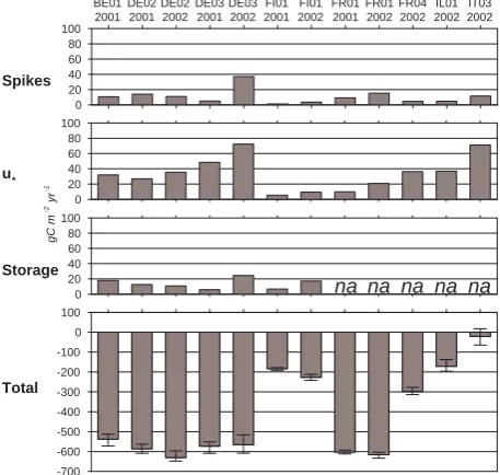
The NEE annual sums obtained with the different combi-nations of the corrections have been used as indicators of the methodological variability to analyze the effect of the differ-ent corrections on the annual balance (Fig. 9a). In the upper three panels the ranges of annual NEE due to each single cor-rection are shown, while in the last plot the mean annual NEE and an error bar indicating minimum and maximum values obtained for each site/year. The mean annual NEE has been calculated using the best storage estimates, filtering the data by the 50% u∗ threshold and applying the spike detection
withz=5.5. Thiszvalue has been chosen instead of the con-ventionally used valuez=4,because the latter is based on the assumption that the data are normally distributed while this is not always the case with the errors in flux data (Richardson et al., 2006).As seen before (Figs. 7, 8), the u∗filtering has
the strongest impact on the data, with generally an effect on the annual NEE of about 40 gC m−2yr−1. DE03 and IT03
are the sites with the highest u∗ filtering impact on the
an-nual NEE (about 70 gC m−2yr−1)while for other sites like FI01 it is very small (the same magnitude as the storage and spike filtering effects), also if the u∗threshold found is one
of the highest (cfr. Fig. 2). Looking to the annual NEE it is possible to see that the uncertainties are between 15 and 100 gC m−2yr−1and in general between 10 and 20% except for IL01 where it is about 30% and IT03 where the effect is strong enough to change the site from sink to source. It is also interesting to note that the uncertainties are of the same mag-nitude of the interannual variability in the four sites where we analyzed two years. This result stresses the importance of a standardized processing to avoid the introduction of arti-ficial between-year and between-site variability that hampers comparative analysis.
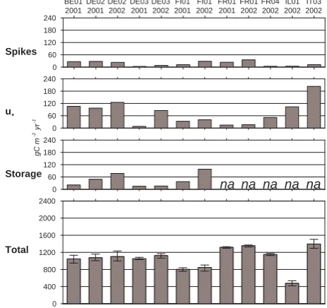
The u∗ filtering has been applied to daytime and
night-time data. However, there is still a debate on this, with part of the scientific community that applies the u∗filtering only
to night-time data (Anthoni et al., 2004; Arain and Restrepo-Coupe, 2005; Haszpra et al., 2005). Figure 9b shows the same plot as Fig. 9a, but in this case we filtered only the night-time data by u∗. It is possible to see that the
uncer-tainty due to u∗ for DE03 dramatically decreases for both
Tot Ust Sto Spa Tot Ust Sto Spa Tot Ust Sto Spa
0 0.1 0.2 0.3 0.4 0.5 0.6 0.7 0.8 0.9 1 1.1 1.2 1.3 1.4 1.5 1.6
gC m
−2
day
−1
Daily 8−daily Monthly
5.96 4.36 2.22 1.92 3.051.47 0.91 0.73 1.060.98 0.26 0.39
0.00 0.00 0.00 0.01 0.03 0.00 0.00 0.00 0.00
[image:9.595.312.544.64.245.2]0.00 0.00 0.00
Fig. 7. Contribution of the different corrections (storage, u∗, spike)
and total effect on daily, 8-daily and monthly NEE across all the sites. Boxplots indicate the range of values obtained applying
re-spectively all the corrections (Tot), the three different u∗thresholds
with the best storage possible and spike 5.5 (Ust), the two
differ-ent storage calculation methods with u∗50% and spike 5.5 (Sto)
and the three different z-values for the spike detection with the best
storage possible and u∗50% (Spa). The red line indicates the
me-dian, the box the inter-quartile range and the dashed lines extending above and below the box show the extent of the rest of the sample (unless there are outliers). In this plot an outlier is a value that is more than 1.5 times the inter-quartile range away from the top or bottom of the box. The minimum and maximum outlier values are displayed as numbers at the top and bottom of the plot.
u* Spike Storage u* + Spike u* + Storage Spike + Storage
DE02 DE03
FI01 BE01
64% 10%
21% 1% 2% 2%
88%
2% 7% 1% 2% 0%
62% 4%
31%
1% 1%1%
58%
5% 37% 0%
Fig. 8. Results of the ANOVA test on the four sites where both the methods to measure the storage flux have been available.
[image:9.595.310.546.434.610.2]BE01 2001 DE02 2001 DE02 2002 DE03 2001 DE03 2002 FI01 2001 FI01 2002 FR01 2001 FR01 2002 FR04 2002 IL01 2002 IT03 2002 0 20 40 60 80 100 0 20 40 60 80 100 0 20 40 60 80 100 -700 -600 -500 -400 -300 -200 -100 0 100
na na na na na
gC m
-2 yr
-1
Spikes
u*
Storage
[image:10.595.49.278.66.283.2]Total
Fig. 9a. Effect of the three different corrections and total uncer-tainty introduced on the annual NEE for the different sites and years.
u∗correction applied to daytime and night-time data. Ranges
cal-culated taking into account 4 spikes detection level (4, 5.5, 7 and
no spike filtering), 3 u∗thresholds (5%, 50%, 95%) and 2 storages
calculation (single point and profile when available, na = not avail-able).
little. The reduction of uncertainty in DE03 can be explained by looking at the percentage of data removed by u∗
filter-ing (Table 2): this is the site with the highest percentage of removed daytime data (up to more than 50%) and with the highest ratio between daytime and night-time data removed (up to 0.82 for DE03 2002 with u∗95%). DE03 is also the
site where the u∗ threshold is the highest and also most
un-certain (Fig. 3). This could be indicative for strong advection occurring also at higher u∗-values at this site, which would
result in u∗filtering being not sufficient under those
condi-tions (Kutsch et al., 20062). For IT03 we do not see a re-duction of uncertainty if we remove only the night-time data with low u∗. This is also partially related to the distribution
of the filtered data between day and night because, unlike DE03, in this site the filtered data are mainly concentrated during night-time. Even though there is still debate on this we suggest, to be more conservative, to apply the u∗filtering
to both daytime and night-time also because the number of data removed during daytime is generally small.
Since the treatment of the NEE data can also have an effect on the partitioning into GPP and TER, we have also anal-ysed the effect of the data treatment on these flux
compo-2Kutsch, W., Kolle, O., Rebmann, C., et al.: Process modelling
and direct measurements of advection reveal uncertainties in flux measurements above a tall forest, Ecological Applications, submit-ted, 2006. BE01 2001 DE02 2001 DE02 2002 DE03 2001 DE03 2002 FI01 2001 FI01 2002 FR01 2001 FR01 2002 FR04 2002 IL01 2002 IT03 2002 0 20 40 60 80 100 0 20 40 60 80 100 0 20 40 60 80 100 -700 -600 -500 -400 -300 -200 -100 0 100
na na na na na
gC m
-2 yr
-1
Spikes
u*
Storage
Total
Fig. 9b. Effect of the three different corrections and total uncer-tainty introduced on the annual NEE for the different sites and years.
u∗correction applied only to night-time data. Ranges calculated
taking into account 4 spikes detection level (4, 5.5, 7 and no spike
filtering), 3 u∗thresholds (5%, 50%, 95%) and 2 storages
calcula-tion (single point and profile when available).
nents (Figs. 9c, d). It seems that the absolute uncertainties introduced into the GPP by the corrections are about twice as high as for the net flux. This is expected since any error on the TER estimate from the night-time data will affect the GPP estimate in the same direction and hence be partially cancelled out when looking at NEE. Moreover, the method-ological variability is higher for TER than for GPP, since day-and night-time TER estimates are affected by data treatment (night-time TER is extrapolated to the day, cf. Reichstein et al., 2005), while the GPP estimates are only during day-time (during night by definition zero). As for NEE the major un-certainty is introduced by the u∗-filtering also for the flux
components. Nevertheless at most sites the range of GPP and TER values obtained by different u∗-thresholds is well below
100 gC m−2yr−1. Since GPP and TER are large fluxes, the relative methodological variability of those fluxes is below 10% in most cases.
4 Conclusions
[image:10.595.307.539.70.284.2]BE01 2001
DE02 2001
DE02 2002
DE03 2001
DE03 2002
FI01 2001
FI01 2002
FR01 2001
FR01 2002
FR04 2002
IL01 2002
IT03 2002
0 60 120 180 240
0 60 120 180 240
0 60 120 180 240
0 400 800 1200 1600 2000 2400
na na na na na
gC m
-2 yr
-1
Spikes
u*
Storage
[image:11.595.307.539.66.284.2]Total
Fig. 9c. Effect of the three different corrections and total uncertainty
introduced on the annual GPP for the different sites and years. u∗
correction applied to daytime and night-time data. Ranges calcu-lated taking into account 4 spikes detection level (4, 5.5, 7 and no
spike filtering), 3 u∗thresholds (5%, 50%, 95%) and 2 storages
cal-culation (single point and profile when available).
Intercomparisons of NEE data sets have been hampered so far by potential differences introduced by non harmonized data processing. We consider the present systematic charac-terization of the joint effects of u∗-filtering, storage
correc-tion, and spike detection on net carbon fluxes and its com-ponents GPP and TER as an important step towards a more standardized processing and away from point estimates to-wards a better quantification of the likely range of integrals of eddy covariance CO2flux data for a given site and year.
We showed the importance of standardized processing that can strongly reduce the margin of uncertainties through a standardized processing also by avoiding inappropriate data treatment (e.g. neglect storage correction or u∗-filtering), but
it is also clear that heuristic methods like the u∗-filtering
con-tain an inherent uncercon-tainty as found by the bootstrapping ap-proach. Large uncertainties in the u∗-thresholds and annual
NEE affected by those at particular sites might also indicate general limits of an insufficiency of the heuristic u∗-filtering
method and standardized data processing at those sites, but it also suggests that this methodology may serve as tool to de-tect this problem, i.e. large uncertainties in the u∗-threshold
associated with large flux uncertainties introduced may be indicative of insufficiency of the u∗-filtering approach. For
a full uncertainty analysis of net CO2fluxes and its
compo-nents estimated by eddy covariance uncertainties introduced by non-captured advection, the gap-filling methods and the flux-partitioning have to be addressed separately. Neverthe-less, from our study we conclude that uncertainties of annual NEE and its components GPP and TER introduced by the
BE01 2001
DE02 2001
DE02 2002
DE03 2001
DE03 2002
FI01 2001
FI01 2002
FR01 2001
FR01 2002
FR04 2002
IL01 2002
IT03 2002
0 60 120 180 240
0 60 120 180 240
0 60 120 180 240
0 400 800 1200 1600 2000 2400
na na na na na
gC m
-2 yr
-1
Spikes
u*
Storage
Total
Fig. 9d. Effect of the three different corrections and total uncer-tainty introduced on the annual TER for the different sites and years.
u∗correction applied to daytime and night-time data. Ranges
cal-culated taking into account 4 spikes detection level (4, 5.5, 7 and
no spike filtering), 3 u∗thresholds (5%, 50%, 95%) and 2 storages
calculation (single point and profile when available).
corrections presented remain well below 100 gC m−2yr−1 and consequently, except for sites where others source of un-certainty dominate, that any spatial or temporal signals or trends that are larger than this number (e.g. continental gra-dients) can be detected by the eddy covariance method de-ployed as a coordinated network.
Acknowledgements. This work has been founded by EC project
CarboeuropeIP (GOCE-CT2003-505572) of the European Commu-nity and the Italian-US joint program CarbiUS (Carbon Regional Balance Italy-USA). We wish to thank FLUXNET and therein D. Baldocchi for having largely created the conditions to build up the community of flux people and the integrated data analysis.
Edited by: A. Neftel
References
Anthoni, P., Freibauer, A., Kolle, O., and Schulze, E.-D.: Winter wheat carbon exchange in Thuringia, Germany, Agric. Forest Meteorol., 121, 55–67, 2004.
Arain, M. A. and Restrepo-Coupe, N.: Net ecosystem production in a temperate pine plantation in southeastern Canada, Agric. Forest Meteorol., 128, 223–241, 2005.
Aubinet, M., Grelle, A., Ibrom, A., Rannik, ¨U., Moncrieff, J.,
[image:11.595.49.279.71.284.2]and Vesala, T.: Estimates of the Annual Net Carbon and Water Exchange of Forest: The EUROFLUX Methodology, Advances in Ecological Research, 30, 114–173, 2000.
Aubinet, M., Chermanne, B., Vandenhaute, M., Longdoz, B., Yer-naux, M., and Laitat, E.: Long term carbon dioxide exchange above a mixed forest in the Belgian Ardennes, Agric. Forest Me-teorol., 108, 293–315, 2001.
Aubinet, M., Heinesch, B., and Longdoz, B.: Estimation of the carbon sequestration by a heterogeneous forest: night flux cor-rections, heterogeneity of the site and inter-annual variability, Global Change Biol., 8, 1053–1071, 2002.
Aubinet, M., Clement, R., Elbers, J. A., Foken, T., Grelle, A.,
Ibrom, A., Moncrieff, J., Pilegaard, K., Rannik, ¨U., and
Reb-mann, C.: Methodology for Data Acquisition, Storage and Treat-ment, in: R. Valentini, Fluxes of Carbon, Water and Energy of European Forests, Springer-Verlag, Berlin, 2003a.
Aubinet, M., Heinesch, B., and Yernaux, M.: Horizontal and
Verti-cal CO2Advection In A Sloping Forest, Boundary-Layer
Mete-orol., 108, 397–417, 2003b.
Baldocchi, D., Falge, E., Gu, L., Olson, R., Hollinger, D., Running, S., Anthoni, P., Bernhofer, C., Davis, K., Evans, R., Fuentes, J., Goldstein, A., Katul, G., Law, B., Lee, X., Malhi, Y., Meyers, T., Munger, W., Oechel, W., Paw, K. T., Pilegaard, K., Schmid, H. P., Valentini, R., Verma, S., Vesala, T., Wilson, K., and Wofsy, S.: FLUXNET: A New Tool to Study the Temporal and Spa-tial Variability of Ecosystem-Scale Carbon Dioxide, Water Va-por, and Energy Flux Densities, Bull. Am. Meteorol. Soc., 82, 2415–2434, 2001.
Bernhofer, C., Aubinet, M., Clement, R., Grelle, A., Gr¨unwald, T., Ibrom, A., Jarvis, P., Rebmann, C., Schulze, E.-D., and Ten-hunen, J.: Spruce Forests (Norway and Sitka Spruce, Including Douglas Fir): Carbon and Water Fluxes and Balances, Ecological and Ecophysiological Determinants, in: R. Valentini, Fluxes of Carbon, Water and Energy of European Forests, Springer-Verlag, Berlin, 2003.
Cook, B. D., Davis, K. J., Wang, W., Desai, A., Berger, B. W., Teclaw, R. M., Martin, J. G., Bolstad, P. V., Bakwin, P. S., Yi, C., and Heilman, W.: Carbon exchange and venting anomalies in an upland deciduous forest in northern Wisconsin, USA, Agric. Forest Meteorol., 126, 271–295, 2004.
Efron, B. and Tibshirani, R. J.: An Introduction to the Bootstrap, Chapman & Hall, New York, 1993.
Falge, E., Baldocchi, D., Olson, R., Anthoni, P., Aubinet, M., Bern-hofer, C., Burba, G., Ceulemans, R., Clement, R., Dolman, H., Granier, A., Gross, P., Gr¨unwald, T., Hollinger, D., Jensen, N.-O., Katul, G., Keronen, P., Kowalski, A., Lai, C. T., Law, B. E., Meyers, T., Moncrieff, J., Moors, E., Munger, J. W., Pilegaard,
K., Rannik, ¨U., Rebmann, C., Suyker, A., Tenhunen, J., Tu, K.,
Verma, S., Vesala, T., Wilson, K., and Wofsy, S.: Gap filling strategies for defensible annual sums of net ecosystem exchange, Agric. Forest Meteorol., 107, 43–69, 2001.
Feigenwinter, C., Bernhofer, C., and Vogt, R.: The Influence of
Ad-vection on the Short Term CO2- Budget in and Above a Forest
Canopy, Boundary-Layer Meteorol., 113, 201–224, 2004. Feigenwinter, C., Heinesch, B., Yernaux, M., Bernhofer, C.,
Eichel-mann, U., Moderow, U., Queck, R., Kolle, O., Hertel, M., Zeri, M., Ziegler, W., Lindroth, A., M¨older, M., Lagergren, F., Mon-tagnani, L., Minerbi, S., Minach, L., Janous, D., Pavelka, M., Acosta, M., and Aubinet, M.: The CarboEurope-IP advection
activities ADVEX’05: A joint effort to improve experimental
and methodological approches of CO2advection measurements,
Geophys. Res. Abstracts, 8, 1607-7962/gra/EGU1606-A-03724, 2006.
Finnigan, J., Aubinet, M., Katul, G., Leuning, R., and Schimel, D.: Report of a Specialist Workshop on “Flux Measurements in Difficult Conditions”, January 26-28, Boulder Colorado, Bull. Am. Meteorol. Soc., in press, 2006.
G¨ockede, M., Markkanen, T., Hasager, C. B. and Foken, T.: Up-date of a Footprint-Based Approach for the Characterisation of Complex Measurement Sites, Boundary-Layer Meteorology, 118, 635-655, 2006.
Goulden, M. L., Munger, J. W., Fan, S. M., Daube, B. C., and Wofsy, S.: Measurements of carbon sequestration by long-term eddy covariance: methods and a critical evaluation of accuracy, Global Change Biol., 2, 169–182, 1996.
Granier, A., Ceschia, E., Damesin, C., Dufrˆene, E., Epron, D., Gross, P., Lebaube, S., Le Dantec, V., Le Goff, N., Lemoine, D., Lucot, E., Ottorini, J. M., Pontailler, J. Y., and Saugier, B.: The carbon balance of a young Beech forest, Functional Ecol., 14, 312–325, 2000.
Grunzweig, J. M., Lin, T., Rotenberg, E., Schwartz, A., and Yakir, D.: Carbon sequestration in arid-land forest, Global Change Biol., 9, 791–799, 2003.
Gu, L., Falge, E. M., Boden, T., Baldocchi, D. D., Black, T. A., Saleska, S. R., Suni, T., Verma, S. B., Vesala, T., Wofsy, S. C., and Xu, L.: Objective threshold determination for nighttime eddy flux filtering, Agric. Forest Meteorol., 128, 179–197, 2005. Haszpra, L., Barcza, Z., Davis, K. J., and Tarczay, K.: Long-term
tall tower carbon dioxide flux monitoring over an area of mixed vegetation, Agric. Forest Meteorol., 132, 58–77, 2005.
Hollinger, D. and Richardson, A. D.: Uncertainty in eddy covari-ance measurements and its application to physiological models, Tree Physiology, 25, 873–885, 2005.
Knohl, A., Schulze, E.-D., Kolle, O., and Buchmann, N.: Large carbon uptake by an unmanaged 250-year-old deciduous forest in Central Germany, Agric. Forest Meteorol., 118, 151–167, 2003. Lee, X., Massman, W. J., and Law, B.: Handbook of
Micromete-orology: A Guide for Surface Flux Measurement and Analysis, Kluwer, Dordrecht, 2004.
Marcolla, B., Cescatti, A., Montagnani, L., Manca, G., Ker-schbaumer, G., and Minerbi, S.: Importance of advection in the
atmospheric CO2 exchanges of an alpine forest, Agric. Forest
Meteorol., 130, 193–206, 2005.
Massman, W. J. and Lee, X.: Eddy covariance flux corrections and uncertainties in long-term studies of carbon and energy ex-changes, Agric. Forest Meteorol., 113, 121–144, 2002.
Moncrieff, J., Mahli, Y., and Leuning, R.: The propagation of errors in long-term measurements of land-atmosphere fluxes of carbon and water, Global Change Biol., 2, 231–240, 1996.
Papale, D. and Valentini, R.: A new assessment of European forests carbon exchanges by eddy fluxes and artificial neural network spatialization, Global Change Biol., 9, 525–535, 2003.
Papale, D. and Reichstein, M.: Centralized quality checks and gap filling used in the CarboeuropeIP Database, AmeriFlux annual meeting 2005, 18–20 October 2005, Boulder Colorado USA. Rambal, S., Joffre, R., Ourcival, J. M., Cavender-Bares, J., and
Ro-cheteau, A.: The growth respiration component in eddy CO2flux
10, 1460–1469, 2004.
Rebmann, C., G¨ockede, M., Foken, T., Aubinet, M., Aurela, M., Berbigier, P., Bernhofer, C., Buchmann, N., Carrara, A., Cescatti, A., Ceulemans, R., Clement, R., Elbers, J. A., Granier, A., Grun-wald, T., Guyon, D., Havrankova, K., Heinesch, B., Knohl, A., Laurila, T., Longdoz, B., Marcolla, B., Markkanen, T., Miglietta, F., Moncrieff, J., Montagnani, L., Moors, E., Nardino, M.,
Our-cival, J. M., Rambal, S., Rannik, ¨U., Rotenberg, E., Sedlak, P.,
Unterhuber, G., Vesala, T., and Yakir, D.: Quality analysis ap-plied on eddy covariance measurements at complex forest sites using footprint modelling, Theoretical and Applied Climatology, 80, 121–141, 2005.
Reichstein, M., Tenhunen, J., Roupsard, O., Ourcival, J.-M., Ram-bal, S., Miglietta, F., Peressotti, A., Pecchiari, M., Tirone, G., and Valentini, R.: Inverse modeling of seasonal drought effects
on canopy CO2/H2O exchange in three Mediterranean
ecosys-tems, J. Geophys. Res., 108, 2003.
Reichstein, M., Falge, E., Baldocchi, D., Papale, D., Aubinet, M., Berbigier, P., Bernhofer, C., Buchmann, N., Gilmanov, T., Granier, A., Gr¨unwald, T., Havr´ankov´a, K., Ilvesniemi, H., Janous, D., Knohl, A., Laurila, T., Lohila, A., Loustau, D., Mat-teucci, G., Meyers, T., Miglietta, F., Ourcival, J.-M., Pumpanen, J., Rambal, S., Rotenberg, E., Sanz, M., Tenhunen, J., Seufert, G., Vaccari, F., Vesala, T., Yakir, D., and Valentini, R.: On the separation of net ecosystem exchange into assimilation and ecosystem respiration: review and improved algorithm, Global Change Biol., 11, 1424–1439, 2005.
Richardson, A. D., Hollinger, D. Y., Burba, G. G., Davis, K. J., Flanagan, L. B., Katul, G. G., William Munger, J., Ricciuto, D. M., Stoy, P. C., Suyker, A. E., Verma, S. B., and Wofsy, S. C.: A multi-site analysis of random error in tower-based measurements of carbon and energy fluxes, Agric. Forest Meteorol., 136, 1–18, 2006.
Ruppert, J., Mauder, M., Thomas, C., and L¨uers, J.: Innovative
gap-filling strategy for annual sums of CO2net ecosystem exchange,
Agric. Forest Meteorol., 138, 5–18, 2006.
Sachs, L.: Angewandte Statistik: Anwendung Statistischer Metho-den, Springer, Berlin, 1996.
Staebler, R. M. and Fitzjarrald, D. R.: Observing subcanopy CO2
advection, Agric. Forest Meteorol., 122, 139–156, 2004. Suni, T., Rinne, J., Reissell, A., Altimir, N., Keronen, P., Rannik,
¨
U., Dal Maso, M., Kulmala, M. and Vesala, T.: Long-term mea-surements of surface fluxes above a Scots pine forest in Hyytiala, southern Finland, 1996–2001, Boreal Environ. Res., 8, 287–301, 2003.
Tedeschi, V., Rey, A. N. A., Manca, G., Valentini, R., Jarvis, P. G., and Borghetti, M.: Soil respiration in a Mediterranean oak forest at different developmental stages after coppicing, Global Change Biol., 12, 110–121, 2006.