Estimation of Parameters of the Kumaraswamy Distribution Based on General Progressive Type II Censoring

Published online December 27, 2014 (http://www.sciencepublishinggroup.com/j/ajtas) doi: 10.11648/j.ajtas.20140306.17

ISSN: 2326-8999 (Print); ISSN: 2326-9006 (Online)

Estimation of parameters of the Kumaraswamy distribution

based on general progressive type II censoring

Mostafa Mohie Eldin

1

, Nora Khalil

2

, Montaser Amein

3

1

Professor in department of Mathematics, faculty of Science, El Azhar University, Cairo, Egypt

2

Lecturer department of Mathematics, faculty of Science, Helwan Universit, Cairo, Egypt

3

Lecturer department of Mathematics, faculty of Science, El Azhar University, Cairo, Egypt

Email address:

[email protected] (N. Khalil)

To cite this article:

Mostafa Mohie Eldin, Nora Khalil, Montaser Amein. Estimation of Parameters of the Kumaraswamy Distribution Based on General Progressive Type II Censoring. American Journal of Theoretical and Applied Statistics. Vol. 3, No. 6, 2014, pp. 217-222.

doi: 10.11648/j.ajtas.20140306.17

Abstract:

In this paper, we produced a study in Estimation for parameters of the Kumaraswamy distribution based on general progressive type II censoring. These estimates are derived using the maximum likelihood and Bayesian approaches. In the Bayesian approach, the two parameters are assumed to be random variables and estimators for the parameters are obtained using the well known squared error loss (SEL) function. The findings are illustrated with actual and computer generated data.

Keywords:

Kumaraswamy’s Distribution, Bayes Estimation, Bayes Prediction, General Progressive Type II Censoring

1. Introduction

The Kumaraswamy distribution is very similar to the Beta distribution, but has the important advantage of an invertible closed form cumulative distribution function. Kumaraswamy (1976, 1978) has showed that the well known probability distribution functions such as the normal, log-normal, beta and empirical distributions such as Johnson’s and polynomial-transformed-normal, etc., do not fit well hydrological data, such as daily rainfall, daily stream flow, etc. and developed a new probability density function known as the sine power probability density function. Furthermore, Kumaraswamy (1980) developed a more general probability density function for double bounded random processes, which is known as Kumaraswamy’s distribution. This distribution is applicable to many natural phenomena whose outcomes have lower and upper bounds, such as the heights of individuals, scores obtained on a test, atmospheric temperatures, hydrological data, etc. Also, this distribution could be appropriate in situations where scientists use probability distributions which have infinite lower and/or upper bounds to fit data, when in reality the bounds are finite. Gupta and Kirmani (1988) discused the connection between non-homogeneous Poisson process (NHPP) and record values. So, the results in this paper may be used for some applied situation such as preventive maintenance.

The paper by Kumaraswamy (1980) proposed a new probability distribution for double bounded random processes with hydrological applications. The continuous part of Kumaraswamy’s distribution has the probability density function (pdf) and the cumulative distribution function (cdf) specified by

( )

₁

(

)

1

1 q

p p

f x = pqx − −x − (1)

and

( )

1

(

1 p

)

q

F x = − −x (2)

respectively, for

0

≤ ≤

x 1

, p > 0 and q > 0. Kumaraswamy (p,q), where p and q are two positive shape parameters. It has many of the same properties as the beta distribution but has some advantages in terms of tractability. This distribution appears to have received considerable interest in hydrology and related areas, see Sundar and Subbiah (1989), Fletcher and Ponnambalam (1996), Seifi et al. (2000), Ponnambalam et al. (2001), and Ganji et al. (2006).

Kumaraswamy distributions are special cases of the three parameter distribution with density

( )

(

)

1 1

1 , 0 1,

,

q p p

p

x x x

B q

γ

γ

−

− _{− ≤ ≤}

Kumaraswamy distributions has special cases, Kumaraswamy (p,1) distribution is the power function distribution, Kumaraswamy (1,p) distributions is the distribution of one minus that power function random variable. Kumaraswamy (1,1) distribution is the uniform distribution.

A further special case of the Kumaraswamy distribution has also appeared elsewhere. The Kumaraswamy (2,q) distribution is that of the” generating variate

{

}

2 2

1 2 when 1, 2

R= x +x x x Follow a bivariate Pearson Type II distribution [K.T. Fang(1990)], Section 3.4.1).

2. Parameter Estimation

Suppose n independent units are placed on life test with corresponding failure times (y1, y2..., ym) being indpendentically distributed with cumulative distribution

function F(y), probability density function f(y), and m prefixed numbers of failures that observed. The scheme (R1, ..., Rm) is the progressively type II censored,

y

i m n; ; be

completely observed times, i=1, 2, …,m. The failure times of the first r units were not observed, at time (r+1)th failure

1 r

R

₊ number of surviving units are withdrawn from the test randomly, and so on. Finally at the time mth failure, the remaining Rm = − −n m Rr+1−Rr+2− −... Rm−1 are withdrawn

from the test.

2.1. ML Estimation

The likelihood function to be maximized when general progressive type II censored sample based on n independent units with F(y) is L(θ).

(

)

(

)

(

)

*

1 1 2

1

( ) ₊, , 1 , , _{+ +} ...

= +

= _ _

∏

_ − _ i < < <

m

r R

r i i r r m

i r

Lθ c F y θ f y θ F y θ y y y (3)

where,

(

) (

) (

)

*

1 1 1

!

1 ... ... 1

! 1 ! + + −

= − − − − − − − +

− − r r m

n

c n R r n R R m

r n r

Using eq. (1) the likelihood function can be expressed as:

(

)

(

)

(

) (

1

(

)

)

( )

(

(

)

)

(

)

( 1 1)

* 1 * 1

1 1

1 1

( ; , ) 1 1 ₊ − 1 − 1 − 1 1 ₊ − 1 + −

= + = +

= − −

∏

− − i = − −

∏

−

i

m m

r R r

q q q m r q q R

p p p p p p p

r i i i r i i

i r i r

L t p q c y pqy y y c pq y y y (4)

The log-likelihood function

ℓ

( ; , )

y p q

_{, is given by:}

(

)

( )

(

(

1

)

)

(

)

( )

(

)

(

)

1 1

( ; , ) constant 1 1 ₊ 1 ( 1) 1 1

= + = +

− + − − + − +

= +

∑

∑

+ − −

ℓ

m m

q

p p

r i i i

i r i r

m r Log

y p q pq rLog y p Log y q R Log y (5)

The ML estimates of p and q can be obtained by maximizing the log-likelihood function, Eq. 5. By taking

derivatives with respect to p and q the MLE are obtained by satisfying the following equations

( )

(

)

(

)

( )

( )

(

(

)

)

1

1 1 1

1 1

1

1

1 1 0

1 1

− +

+ + +

= + = +

+ − −

= + + − − + +

− −

∑

∑

=

ℓ

q p p

m m

r r r p

i i i i

q p

i r i r r

qrLog y y

m r

Log Log q R y

y y

p y

p y

δ δ

(

)(

)

(

)

(

)

(

)

1 1

1 1

1 1

1 1

1 1

0

+ +

= + +

− −

−

= − + + −

− −

∑

=

ℓ

q p p _m

r r _p

i i q

p

i r r

rLog y y

m r

R y

q q _y

δ δ

The above system is nonlinear, but can be easily solved using numerical techniques.

2.2. Bayes Estimation of the Unknown Parameter(s)

In this subsection we consider the Bayes estimation of the unknown parameter(s). We will assume that the parameters p and q of the Kumaraswamy’s distribution are random variables with a joint bivariate prior density function that was first suggested by Al-Hussaini and Jaheen (1995) as,

(

p q,

)

g q p g1

(

|

) ( )

2 p

π

= (6)

where

(

)

₍

₎

1

1 | ₁ 1 , -1, 0

pq

p

g q p q e

α

α γ

α α γ

α γ

+ ₋

+

= > >

Γ + (7)

is the gamma conjugate prior. This prior was first introduced by Papadopoulos (1978) and was also used later on by Al-Hussaini and Jaheen (1992). The prior of p is

( )

_{( )}

1

2 , 0, 0

p

p

g p e

δ

β

δ δ β

δ β

− ₋

= > >

which is the gamma (δ, β) density.

Substituting (6) and (7) in (5) we obtain the bivariate prior density of p and q given as

(

p q,

)

pδ α αq exp

(

p

(

1 q

)

)

π

_∝ + ₋

β

₊

γ

(9)

where α > −1, β, δ and γ are positive real numbers.

From (3) and (9), the joint posterior distribution is given by

(

)

(

) (

) ( )

(

) (

) ( )

1 2

1 2

0 0

| , |

, | =

| , |

L data p q g q p g p

p q data

L data p q g q p g p dpdq

π _{∞ ∞}

∫ ∫

(

)

(

) (

) ( )

(

) (

) ( )

1 2

1 2

0 0

| , |

, | =

| , |

L data p q g q p g p

p q data

L data p q g q p g p dpdq

π _{∞ ∞}

∫ ∫

(

)

(

)

( ) ( ( ) )

_{( )}

(

)

(

)

( ) ( ( ) )

( )

(

)

1

1 1

1

1 1

1 ln 1 1 ln 1

ln 1 1

1 ln 1 1 ln 1

ln 1 1

0 0

, |

=

+

= + = +

+

= + = +

  _{+ + − − − +}

− −

 

+ + − + −  

 

∞ ∞ _{− −  + + − − − +}

+ + − + −  

∑

∑

∑

∑

∫ ∫

m m

q p

p

i i i

r

i r i r

m m

q p

p

i i i

r

i r i r

q

p y q R y p

r y

m r m r

q

p y q R y p

r y

m r m r

p

q

e

e

p q data

p

q

e

e

dpdq

γ β

α δ α

γ β

α δ α

π

(

)

(

)

( ) ( ( ) )

( )

(

)

(

) (

)

1

1 1

1

ln 1 1 ln 1

ln 1 1

, |

=

1

0,1, 0, 0

+

= + = +

 _{− −}  _{+ + − − − +}

 

+ + − + −  

∑

∑

Γ

+ − +

m m

q p

p

i i i

r

i r i r

q

p y q R y p

r y

m r m r

p

q

e

e

p q data

m

r

γ β

α δ α

π

α

ψ

(10)

Where

(

)

( )

( ) ( )

(

)

(

)

(

)

1 1

ln ln 1

0 0

1 1

, , , 1

1 ln 1 ln 1

m m

z

i i

i r i r

z d y y m r a

r _r r

m r c

j m

j _{z z}

i i r

i r

z e dz

a c d f

z _{R y j y f}

α δ

α

ψ

γ

= + = +

 

 

−_ − _− −

∞ + + − +  

+ − + =

+ = +

∑ ∑

 

= −  

  

− + 

 

 − − − + 

∑

∫

∑

If the loss function is the well known squared error loss function, the Bayes estimators for the parameters p and q are the given by their marginal posterior expectations as

(

)

₍

(

1,1, 0, 0

)

₎

ˆp =E |

0,1, 0, 0

B p y

ψ ψ

=

And

(

) (

) (

₍

0, 2, 0, 0

₎

)

ˆ =E | 1

0,1, 0, 0

B

q q y m α r ψ

ψ

= + − +

3. Numerical Examples

A simulation study with real data is conducted in order to compare the performances between MLE and Bayes estimator.

3.1. Illustrative Examples

Example 1(real data)

In order to illustrate the findings of Sects. 2 and 3 two examples are given. The former is a real data set obtained from the Shasta reservoir in California while the latter example uses simulated data set. In both examples the mathematical package was used to obtain the estimates of the parameters a and b and Bayes predictive estimates.

The first example deals with the monthly water capacity data from the Shasta reservoir in California, USA and were

taken for the month of February from 1991 to 2010, http://cdec.water.ca.gov/reservoir_map.html. The maximum capacity of the reservoir is 4552000 AF and the data were transformed to the interval [0, 1].

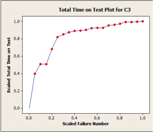
Fig. 1. The empirical hazard function.

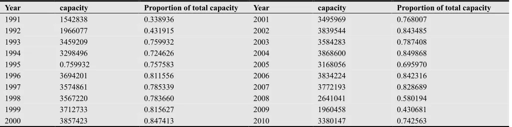
Table 1. Monthly capacity for August and proportion of total capacity for Shasta reservoir.

Year capacity Proportion of total capacity Year capacity Proportion of total capacity

1991 1542838 0.338936 2001 3495969 0.768007

1992 1966077 0.431915 2002 3839544 0.843485

1993 3459209 0.759932 2003 3584283 0.787408

1994 3298496 0.724626 2004 3868600 0.849868

1995 0.759932 0.757583 2005 3168056 0.695970

1996 3694201 0.811556 2006 3834224 0.842316

1997 3574861 0.785339 2007 3772193 0.828689 1998 3567220 0.783660 2008 2641041 0.580194 1999 3712733 0.815627 2009 1960458 0.430681 2000 3857423 0.847413 2010 3380147 0.742563

The 20 values were used to verify that the transformed data follow Kumaraswamy’s distribution, by examine the empirical hazard function of the observed data by applying the scaled Total Time on Test (TTT) plot, see Aarset (1987). This provides a very good idea about the shape of the hazard function of a distribution. For a family with the survival function s y

( )

= −1 F y

( )

, The scaled TTT with

( ) ( ) ( )

1

0

F u

H− u =

∫

s y dy _{define for}

0

< <

u

1

_is

( )

( )

( )

1

1

1

H u

g u H

−

−

= .

The corresponding empirical version of the scaled TTT

transform is given by

( )

( )

_{( )}

( ) ( ) ( ) ( )

1

1 1

1

1

r

i r

n i

n n

n

i i

y n r y H r n

g r n H

y

−

= −

=

 

+ −

 

 

= =

∑

∑

,

where y_{( )}i denotes the i-th order statistic of the sample. It has

been shown by Aarset (1987) that the TTT transform is convex (concave) if the hazard rate is decreasing (increasing); and for bathtub (unimodal) hazard rates, the scaled TTT transform is first convex (concave) and then concave (convex). The plot of the scaled TTT transform of the data, Fig. 1, indicates that the empirical hazard function is increasing and therefore, it is reasonable to use the Kumaraswamy’s distribution to analyze the data.

We also wanted to check by using the Kolmogorov_Smirnov (K_S) statistic whether the Kolmogorov–Smirnov test showed that indeed the observations follow the Kumaraswamy’s distribution (p value > 0.2).

Failure time vector Y= (y4 , …, y9) and censoring scheme R= (R4, …, R9),r=3.

i 1 2 3 4 5 6 7 8 9

Yi - - - 0.430681 0.431915 0.580194 0.695970 0.724626 0.785339

Ri - - - 1 2 0 4 2 2

MLE, posterior mean, median and mode of the parameter

Parameter MLE Posterior mean Posterior mode Posterior median

p 3.38005 3.2005 3.16566 3.1436

q 1.34034 1.15226 1.09477 1.0563

Example 2 (generation data)

The following data is general progressively type II censored sample from Kumaraswamy distribution (p = 3, q = 2) was simulated by using n=60, r=9, m=29 and censored scheme [Ri= {4,1,1,1,1,3,1,0,3,0,2,0,3,2,3,0,0,3,2,1},

i=r+1, …,m]: 0.4520, 0.4654, 0.4702, 0.4925, 0.5052, 0.5182, 0.5284, 0.5528, 0.5654, 0.5890, 0.6274, 0.6402, 0.6696, 0.6812, 0.7056, 0.7092, 0.7323, 0.7566, 0.7871, 0.8223.

MLE, posterior mean, median and mode of the parameter

Parameter MLE Posterior mean Posterior mode Posterior median

p 3.08216 3.0326 2.88523 2.7625

q 1.8516 1.6276 1.60599 1.4276

3.2. Monte Carlo Simulations

In the following, Monte Carlo simulation study is conducted in order to compare the performance of the Bayes estimator with MLE for different sample sizes and censoring schemes. We generate progressively type II censored samples

from Kumaraswamy distribution with parameter p=3, q=2, different combinations of the effective sample size

(

)

m′ = m r− and different progressive censoring schemes (Rr+1, Rr+2 ,..., Rm). The different progressive censoring

1 1

* 0, , * 0

2 2

m m

n m

′− ′−

 ₋ 

 

  and III)

(

m′ −1* 0,n m−

)

. For simplicity in notation, we denote these censoring schemes, for example, by (3*0,1,5) which represents the censoring scheme ( R4= 0, R5 = 0, R6= 0, R7 = 1, R8 = 5) for fixed r = 3.

The programs were written by Mathematica 9. In computing the estimates we generated 1000 samples from the

Kumaraswamy distribution, and we replicated the process 1000 times. The averages and mean squared errors (MSE) in parentheses of estimators of p and q are presented in Tables 2 and 3, respectively. For prior information we have used prior1 with α=1, γ =2, δ =1, β =1.

Table 2. Average estimates of p and the associated MSEs when r=3.

n m Effective sample sizem′ (Rr+1, Rr+2 ,..., Rm) Censoring schems MLE Bayes Prior1

20 10 7

(6*0,10)

(3*0,10,3*0)

(0, 2*1,2,1,3 )

3.1131 (0.2662) 3.0516 (0.3159)

3.1593

(0.3305)

3.18885 (0.3062) 3.09802 (0.2809)

3.2018

(0.3053)

12 9

(8*0,8)

(4*0,8, 4*0)

(2,0,2,0,2,0,2,2*0)

3.02529 (0.1200) 3.09034 (0.3073) 3.10669 (0.3453)

2.9806 (0.2230) 3.17932 (0.2960) 3.19834 (0.3526)

30 10 7

(6*0,20)

(3*0,20, 3*0)

(5,0,5,0,5,0,5)

3.01308 (0.17909) 3.04555 (0.19109) 3.03692 (0.18950)

3.17069 (0.18989) 3.18085 (0.18782) 3.16 (0.1933)

12 9

(8*0,18)

(4*0,18, 4*0)

3.04414 (0.1761) 3.02868 (0.211869)

3.22823 (0.2244) 3.18064 (0.2013)

20 17

(16*0,10)

(8*0,10, 8*0)

(2,0,3*1,6*0,2*1,3*0,3)

3.01585 (0.13514) 3.00253 (0.1609) 3.00044 (0.1531)

3.05194 (0.1363) 3.01027 (0.1556) 3.20177 (0.2317)

Table 3. Average estimates of q and the associated MSEs when r=3.

n m Effective sample sizem′ (Rr+1, Rr+2 ,..., Rm) Censoring schems MLE Prior1

20 10 7

(6*0,10)

(3*0,10,3*0)

(0, 2*1,2,1,3 )

2.13186 (0.17392) 2.15666 (0.22698)

2.1697

(0.2462)

2.0108 (0.2042) 2.0717 (0.2024)

2.0343

(0.2133)

12 9

(8*0,8)

(4*0,8, 4*0)

(2,0,2,0,2,0,2,2*0)

2.06577 (0.15831) 2.11246 (0.2005) 2.11698 (0.1766)

2.06063 (0.1782) 2.08378 (0.2572) 2.08138 (0.25484)

30 10 7

(6*0,20)

(3*0,20, 3*0)

(5,0,5,0,5,0,5)

2.02441 (0.2238) 2.0848 (0.2157) 2.07875 (0.2237)

2.12304 (0.2782) 2.09572 (0.2142) 2.1284 (0.31579)

12 9

(8*0,18)

(4*0,18, 4*0) (4,0,4,0,4,0,4,0,2)

2.00134 (0.178693) 2.08847 (0.200834)

2.12667 (0.302296) 2.15622 (0.283017)

20 17

(16*0,10)

(8*0,10, 8*0)

(2,0,3*1,6*0,2*1,3*0,3)

2.04804 (0.1069) 2.05152 (0.1399) 2.06452 (0.1571)

4. Conclusion

In this paper we have considered Estimation problems for parameters of the Kumaraswamy based on progressive Type-II censored data by using Maximum Liklehood Estimation and the Bayesian inference. The prior belief of the model is represented by the independent gamma conjugate priors on the shape parameters. The squared error loss function is used as it is appropriate when large errors of the estimation are considered to be more serious compared to other loss functions. We used Mathematica program to generate the samples and bisection method to compute the estimated parameters. The details have been explained using a real life example and computer generated data. Simulation study was conducted in order to compare the performance of the Bayes estimators with MLE for different sample sizes and censoring schemes , it was seen that the behavior of the MLE and Bayes estimates depends on the kind of censoring schemes, and the results were summarized as follow:

i. Comparing the behavior of MLE and Bayes estimators: where when used random censoring schemes the MLE and Bayes estimators were almost same values in terms of MSE; however, it was seen that the Bayes estimators were better than their corresponding MLEs when used the following censoring schemes

1 1

* 0, , * 0

2 2

m m

n m

′− ′−

 ₋ 

 

  and the MLEs were better than their corresponding the Bayes estimators when used the following censoring schemes

(

m′ −1* 0,n m−

)

. An important problem will be to extend these results for other censoring schemes such as Type-I, hybrid censoring schemes. The work is in progress.

ii. behavior of the MLE:

the behavior of MLE in censoring scheme number I was better than number II, III.

iii. behavior of Bayes estimators:

the different kind of censoring schemes behavior of does not effect on Bayes estimators behavior.

References

[1] Aarset, M.V (1987) How to identify a bathtub hazard function. IEEE Transactions on Reliability 36: 106–108.

[2] Al-Hussaini EK, Jaheen ZF (1992) Bayesian estimation of the parameters, reliability and failure rate functions of the Burr Type XII failure model. J Stat Comput Simul 41:37–40 [3] Chansoo Kim, Keunhee Han (2009) Estimation of the scale

parameter of the Rayleigh distribution under general progressive censoring. Journal of the Korean Statistical Society 38: 239_246

[4] Fletcher SC, Ponnamblam K (1996) Estimation of reservoir yield and storage distribution using moments analysis. J Hydrol 182:259–275

[5] Gupta RC, Kirmani SNUA (1988) Closure and monotonicity properties of nonhomogeneous Poisson processes and record values. Probab Eng Inf Sci 2:475–484

[6] K.T. Fang, S. Kotz, K.W. Ng, Symmetric Multivariate and Related Distributions, Chapman and Hall, London, 1990. [7] Kumaraswamy P (1976) Sinepower probability density

function. J Hydrol 31:181–184

[8] Kumaraswamy P (1978) Extended sinepower probability density function. J Hydrol 37:81–89

[9] Kumaraswamy P (1980) A generalized probability density function for double-bounded random processes. J Hydrol 46:79–88

[10] Ponnambalam K, Seifi A, Vlach J (2001) Probabilistic design of systems with general distributions of parameters. Int J Circuit Theory Appl 29:527–536

[11] Seifi A, Ponnambalam K, Vlach J (2000) Maximization of manufacturing yield of systems with arbitrary distributions of component values. Ann Oper Res 99:373–383