Statistical modelling of agrometeorological time series by exponential smoothing

Statistical modelling of agrometeorological time series by exponential smoothing

2_{INRES, University of Bonn, 53115 Bonn, Germany}

3_{Institute of Agrophysics, Polish Academy of Sciences, Doświadczalna 4, 20-290 Lublin, Poland}

Received March 12, 2015; accepted November 24, 2015

*Corresponding author e-mail: pbaranow@ipan.lublin.pl A b s t r a c t. Meteorological time series are used in model-ling agrophysical processes of the soil-plant-atmosphere system which determine plant growth and yield. Additionally, long-term meteorological series are used in climate change scenarios. Such studies often require forecasting or projection of meteoro-logical variables, eg the projection of occurrence of the extreme events. The aim of the article was to determine the most suitable exponential smoothing models to generate forecast using data on air temperature, wind speed, and precipitation time series in Jokioinen (Finland), Dikopshof (Germany), Lleida (Spain), and Lublin (Poland). These series exhibit regular additive seasonality or non-seasonality without any trend, which is confirmed by their autocorrelation functions and partial autocorrelation functions. The most suitable models were indicated by the smallest mean absolute error and the smallest root mean squared error.

K e y w o r d s: exponential smoothing, meteorological time series, statistical forecasting,

INTRODUCTION

Meteorological time series are an important source of information for agricultural planning. Basically, every farm

operation and the process of plant growth and develop

-ment as well as the yield of a crop are strongly affected by

weather conditions (Porter and Semenov, 2005; Pirttioja et

al., 2015). Therefore, meteorological time series are

essen-tial for crop modelling while forecasting of meteorological

quantities is indispensable for scheduling agrotechnical measures such as fertilizer application (Asseng et al., 2012), irrigation (Magno et al., 2014), harvesting (Toscano et al.,

2014; Trnka et al., 2014). Modelling and forecasting of

meteorological time series improve our understanding of the variation of climatic conditions at varying scales in order to assess the effects of climate change on crop

pro-duction (Smith et al., 2007). For instance, forecasts can be

used to assess or to anticipate potentially hazardous weath

-er extremes such as frosts, droughts, high winds (Schlenk-er

and Roberts, 2006).

Two distinct approaches exist in forecasting and projec

-tion of meteorological elements: dynamical-physical models

based on the laws of physics, including global circulation

models (GCMs) used for long-term climate projections, and statistical models estimated directly from observa-tions that are used for short-term predicobserva-tions (McSharry,

2011). The first group of models facilitates projection of the effects of climate change. However, these models are based

on understanding the interactions between mass and ener

-gy exchange between oceans, atmosphere, and biosphere, which are still not sufficiently acknowledged. On the other

hand, the quality of forecasts based on statistical models

strongly depends on the extent to which the future resem

-bles the past. Representative historical data are therefore crucial for proper construction of such models.

Key meteorological time series are air temperature, humi-

dity and pressure, wind speed, precipitation, and solar radia-tion, which are automatically measured within meteorolo-gical stations with relatively high frequency and accuracy. Long-term meteorological records from around the world

are available nowadays, giving a good background for test

-ing various statistical forecast-ing methods that try to build a model of the process that is to be predicted. While the idea of forecasting is to use an elaborated model on the va- lues of the series to predict future ones, the meteorological forecasting techniques further depend on the time scale in

question and the type of the series (Baranowski et al., 2015;

Meehl et al., 2009; Smith et al., 2007).

Methods used in statistical forecasting of meteoro-logical time series include analyses of simple exponential

smoothing, random walk, moving average, autoregressive

integrated moving average (ARIMA), and artificial intel

-ligence techniques such as Fuzzy Logic, Multi-Layered Perceptrons, Radial Basis Functions, Logistic Regression,

and Recurrent Neural Networks (Bilgili, 2007; Chan et

al., 2006; Dong et al., 2013; Ghiassi et al., 2005; Reikard,

2009). Additionally, the hybrids of different methods are

used to improve the forecasting accuracy. Although some of these methods represent a very sophisticated level of

complexity, it was shown during model comparisons that

statistically sophisticated or complex methods did not ne- cessarily provide more accurate forecasts than simpler ones (Makridakis and Hibon, 2000).

The exponential smoothing methods play a special role in forecasting of meteorological time series and they are still being developed and improved (Gardner, 2006). A total

of fifteen methods can be distinguished as the main frame

-work of the family of the exponential smoothing methods. Additionally, a state space framework was elaborated,

which can be applied to all the exponential smoothing mod

-els and which allows computation of prediction intervals,

likelihood, and model selection criteria (Hyndman and

Khandakar, 2008; Hyndman et al., 2002).

The aim of this paper is to compare statistical short-time

forecasting of air temperature, precipitation and wind speed

using exponential smoothing on the basis of 31 years time series originating from four different locations in Europe.

MATERIALS AND METHODS

Four study sites were selected according to the fol

-lowing criteria in order to offer a cross-section of climatic conditions in Europe as well as their shifts under climate

change. In order to represent the contrasting climatic

con-ditions with a minimum number of sites, it was decided

to choose sites for northern, central, and southern Europe.

Jokioinen in Finland was chosen for northern Europe and

Lleida in Spain for southern Europe. For central Europe,

two sites were chosen: Dikopshof located in the west part

of Germany and Lublin in the east part of Poland. The four sites represent boreal, Atlantic central, continental, and

Mediterranean south climates. The principal characteristics of these sites and their agro-climatic conditions are sum-marised inTable 1.

Jokioinen site has a subarctic climate that has severe

winters, no dry season, cool, short summers, and strong sea-sonality (Köppen-Geiger classification: Dfc). Lleida has a semi-arid climate with Mediterranean-like precipitation

patterns (annual average of 369 mm), foggy and mild win

-ters, and hot and dry summers (Köppe-Geiger classification:

BSk). Dikopshof represents a maritime temperate climate

(Köppen-Geiger climate classification: Cfb). There is

sig-nificant precipitation throughout the year in the German site. Lublin site has a warm summer continental climate (Köppen-Geiger climate classification: Dfb). The weather

time series in all sites were measured with standard equip

-ment, comparable for all stations. Three variables were

considered in the present study: air temperature,

precipita-tion, and wind speed. Datasets were collected on a daily basis from January 1st 1980 to December 31st 2010 (11 322 days). For Jokioinen, wind speed was measured at 10 m height and was converted to a height of 2 m assuming the

logarithmic wind profile of Allen et al. (1998, their eq. 47).

For Lleida, the wind speed time series had gaps of 82 days in autumn 1986 and global radiation data had gaps of 48 days (11 days in September 1988 and 37 days in spring 1990). These gaps were filled by taking the absolute values

of the associated grid cell in the ERA-interim dataset. The descriptive statistics of the meteorological time series are presented in Table 2. The highest mean and me- dian values of air temperature in the period of 31 years

were observed at Lleida station and the lowest at Jokioinen

station. The parameters of skewness and kurtosis of the ana

-lysed time series give information about differences in their statistical distributions. Air temperature is characterized by

negative skewness and small kurtosis, which inform us that

this distribution is left-tailed and has a more rounded peak

and thinner tails compared to the wind speed distribution, characterized by positive skewness and larger kurtosis.

Completely different distribution shape can be observed

for precipitation, with higher positive skewness and very

large kurtosis values for all the stations. This means that this distribution is strongly right-tailed and has a very sharp peak and fat tail.

T a b l e 1. The principal characteristics of sites and their agro-climatic conditions

Site Jokioinen Dikopshof Lublin Lleida

Country Finland (FI) Germany (DE) Poland (PL) Spain (ES)

Latitude (o_{N) 60}o_{48’ 50}o_{48’29’’ 51}o_{14’55’’ 41}o_42’

Longitude (o_{E) 23}o_{30’ 6}o_{57’7’’ 22}o_{33’37’’ 1}o_6’

Altitude (meters) 104 60 194 337

A time series is an ordered sequence of values of a va- riable at equally spaced time intervals, eg hourly

tem-peratures at weather stations. The main aim of time series

modelling is to carefully collect and rigorously study the past observations of a time series to develop an appro-

priate model which describes the inherent structure of the

series. This allows explaining the data in such a way allow

-ing prediction, monitor-ing, or control. A common method used to study time series is the exponential smoothing. The idea of exponential smoothing is to smooth the noise out of the original series and to use the smoothed series in forecasting future values of the variable of interest. The exponential smoothing is a smoothing technique used to reduce irregularities such as a long-term direction and

random fluctuations with known periodicity in time series data, thus providing a clearer view of the true underlying

behaviour of the series. It also provides an effective means of predicting future values of the time series (forecasting).

In exponential smoothing, forecasts are weighted combina

-tions of past observa-tions, with recent observa-tions given relatively more weight than older observations. The name ‘exponential smoothing’ reflects the fact that the weights

decrease exponentially as the observations get older. The main advantage of the exponential smoothing methods is

their robustness that allows a fast and efficient implementa

-tion of the technique together with the descriptive and the

inferential statistics.

Exponential smoothing was introduced and developed by Brown (1959, 1963). Independently, Holt (2004) develo-ped a similar exponential smoothing method with a different

approach for smoothing seasonal data. Since then, several

authors (Gardner, 1985; Hyndman et al., 2002, 2008; Muth,

1960; Winters, 1960) have worked to develop exponential smoothing within a statistical framework.

Taking into account the pattern of the time series

con-sidered in this paper, we focus on two models: the simple exponential smoothing and the exponential smoothing with no-trend and with seasonality which are denoted as the

(N,N) model and the (N,A) model, respectively (Hyndman

et al., 2008), where the pair (*,*) stands for a possible trend

and seasonal combinations. It should be noted that in the (*,*) notation A stands for the additive component and N stands for none.

The (N,N) model is used for data patterns without cyclic

variation or pronounced trend. This model for a given time series y₁, ..., y_n is given by the equation:

l_t=α y_t + (1-α) l_t-1, (1)

where: l_t denotes an exponential smoothed value of the

series at time t and a is a smoothing weight. The method

of simple exponential smoothing (N,N) takes the forecast for the previous period and adjusts it using a forecast error.

Hence, the new forecast is simply the old forecast plus an

adjustment for the error that occurred in the last forecast.

T a b l e 2. Descriptive statistics of the whole daily 31 years meteorological time series from 6 stations in Germany (DE), Finland (FI), Poland (PL), and Spain (ES)

Meteorological

variable Site Mean Min Max Std Median Skewness Kurtosis

Precipitation (mm day-1₎

Jokioinen (FI) 1.7 0.0 79.1 3.9 0.1 5.0 49.3

Dikopshof (DE) 1.7 0.0 75.4 3.8 0.0 4.5 38.1

Lublin (PL) 1.5 0.0 61.6 3.9 0.0 5.7 49.7

Lleida (ES) 0.9 0.0 83.6 3.8 0.0 7.2 75.7

Wind speed (m s-1₎

Jokioinen (FI) 2.3 0.0 7.7 1.0 2.6 0.5 3.5

Dikopshof (DE) 2.6 0.2 9.4 1.3 2.4 1.1 4.8

Lublin (PL) 3.0 0.0 17.4 1.8 3.1 1.5 6.5

Lleida (ES) 2.6 0.3 17.8 1.7 2.2 2.0 9.2

Air temperature (°C)

Jokioinen (FI) 4.6 -33.4 25.0 9.3 4.7 -0.4 2.8

Dikopshof (DE) 10.2 -16.8 28.9 6.8 10.5 -0.2 2.5

Lublin (PL) 8.7 -22.8 28.3 8.8 9.1 -0.2 2.4

Lleida (ES) 15.0 -8.3 33.1 7.6 14.7 0.0 2.1

The (N,A) model is used for data which do not indi -cate any trend and experience regular changes repeated

with nearly the same pace and intensity. This model for

given time series y₁, ..., y_n is well described by the system

of equations:

l_t=αy_t - s_t-m+(1-α) l_t-1, (2)

s_t = δ(y_t - l_t-1)+(1-δ) st-m, (3)

where: s_t denotes a smoothed seasonal component of the

series at time t, m is the length of seasons, and δ is a

season-al weight. The smoothing Eqs (1), (2), and (3) determine how the smoothing value changes as time progresses. The smoothing weights determine the contribution of the

pre-vious smoothing value to the current smoothing value. At the beginning, the smoothing process computes the smoothing value for time t = 1. However, this computation

requires an initial estimate of the smoothing value at time t = 0. An appropriate choice for the initial smoothing state S0 is computed as the mean for all values included in

com-plete seasonal cycles.

Smoothing weight α and seasonal weight δ take values

between zero and one. If α=1, then the previous

observa-tions are ignored entirely. If α=0, the current observation is ignored entirely, and the smoothed value consists entirely of the previous smoothed value. Values of α in-between

produce intermediate results.

If δ = 0, then the seasonal component for a particular point in time is predicted to be identical to the predicted seasonal component for the respective time during the

previous seasonal cycle, which in turn is predicted to be

identical to that from the previous cycle, and so on. Thus, a constant unchanging seasonal component is used to generate the one-step-ahead forecasts. If δ = 1, then the

sea-sonal component is modified ‘maximally’ at every step by

the respective forecast error.

Suppose we have observed data up to and including

time t-1 and we want to forecast the next value y_t of our time series. If the forecast is denoted by ŷ_t+h|t, then the fore-cast error e_t is found to be y_t-ŷ_t+h|. The forecast for the next

period is ŷ_t+h|t=lt for the (N,N) model and ŷt+h|h= lt + st-m+h for the (N,A) model.

A visual check of the accuracy of forecasts is often the

most powerful method for determining whether or not the current exponential smoothing model fits the data. We can

also examine autocorrelation function (ACF) and partial autocorrelation function (PACF) plots. The ACF plot is a bar

chart of the coefficients of correlation between a time series

and lags of itself. The PACF plot is a plot of the partial

cor-relation coefficients between the series and lags of itself.

To determine the optimum parameters of the chosen

model, we use the mean absolute error (MAE) and the root

mean squared error (RMSE):

,| 1

= _n

∑

MAE (4)

, 1

=

∑

=

n t et n

RMSE (5)

where: n is the number of periods of time.

The MAE and the RMSE can be used together to diag-nose the variation in the errors in a set of forecasts. The

MAE is the average over the verification sample of the

absolute values of the differences between forecast and the

corresponding observation. The RMSE is the square root of

the average squared values of the differences between the

forecast and the corresponding observation. Those errors have the same units of measurement and depend on the

units in which the data are measured.

The chosen model was run by using computer software

STATISTICA, Stat Soft Inc., USA. The implementation of the exponential smoothing methods in STATISTICA

fol-lows closely the survey of techniques presented by Gardner

(1985), who proposed a ‘unified’ classification of expo

-nential smoothing methods. The parameters α and δ of the (N,A) model and the parameter α of the (N,N) model

were selected by a grid search of the parameters space and the accuracy was chosen as a criterion for determination thereof. The values of the parameters were systematically evaluated by starting with value α = 0.1 and δ = 0.1 with

increments of 0.1. Then α and δ were chosen to produce

the smallest MAE and RMSE for the residuals (ie observed values minus one-step-ahead forecasts).

The majority of plots and the basic statistics of the time

series were completed with the use of RStudio integrated development environment for R version 0.97.551 (R Core Team, 2014).

RESULTS AND DISCUSSION

The visual analysis of the air temperature time series

and their decomposition plots (not shown) do not indicate any long-term trends, but they have regular fluctuations which are repeated from year to year with about the same

timing and level of intensity. The ACF and PACF plots

indicate seasonal temperature patterns without trends at all four sites (Fig. 1). A seasonal character with no trend was also observed for wind speed (Fig. 2). This implies that the

best exponential smoothing model for air temperature and

wind speed is the additive seasonal model (N,A).

The results obtained for air temperature series are

pre-sented in Table 3. It can be observed that the best-fitting

model for the temperature series from each of the

consid-ered sites was characterized by the same pair of parameters a=0.9 and δ = 0.1. This means that changes in air

tempera-ture time series have the same natempera-ture and pattern for the

considered sites. Similarly, we obtained δ = 0.1 for all the

wind speed models, but the a value for Dikopshof, Lublin,

and Lleida wind speed time series that generates the small

smallest RMSE (Table 4). This low value of the seasonal

parameter δ suggests that the air temperature and wind

speed data are not strongly affected by seasonal factors. The high value of the smoothing parameter a indicates that

the fluctuation of the air temperature is large and the low

values of a show small variablity in wind speed data. The smoothed value calculated for the final period in each of the

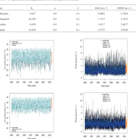
finally selected models can be used for forecasting future statistics. Figure 3 presents the comparison between real

and annual forecast of the air temperature in Jokioinen and

Lleida, respectively, obtained using the (N,A) model with

parameters a=0.9 and δ = 0.1. The real values and annual forecast of the wind speed in Dikopshof and in Lublin are shown in Fig. 4.

Fig. 1. ACF and partial ACF plots for air temperature time series from: A and B – Lleida, Spain; C and D – Jokioinen, Finland; stations.

T a b l e 3. Exponential smoothing parameters for mean air temperature ((N,A) model)

Site S0 α δ MAE (°C) RMSE (°C)

Jokioinen 4.657 0.9 0.1 2.0482 2.7626

Dikopshof 10.250 0.9 0.1 1.7113 2.1932

Lublin 8.670 0.9 0.1 1.9117 2.4877

Lleida 15.050 0.9 0.1 1.5772 2.0230

T a b l e 4. Exponential smoothing parameters for wind speed ((N,A) model)

Site S0 α δ MAE (m s-1) RMSE (m s-1)

Jokioinen 4.657 0.9 0.1 2.0482 2.7626

Dikopshof 10.250 0.9 0.1 1.7113 2.1932

Lublin 8.670 0.9 0.1 1.9117 2.4877

Lleida 15.050 0.9 0.1 1.5772 2.0230

Fig. 3. Smoothed time series and annual forecasting of air temper-ature ((N,A) model) in Jokioinen (upper plot) and Lleida (lower plot).

Fig. 4. Smoothed time series and annual forecasting of wind speed ((N,A) model) in in Dikopshof (upper plot) and Lublin (lower plot).

W

ind speed (m s

-1)

W

ind speed (m s

A quite different situation was found for precipitation

time series. The analysis of the time series courses and the ACF and PACF plots revealed that the (N,N) model should

be applied to Dikopshof and Lleida time series, which do

not demonstrate a trend or seasonality, and the (NA) model should be applied to Lublin and Jokioinen time series,

which do not demonstrate a trend but show seasonality

(Fig. 5). The parameters that produced the smallest MAE or RMSE are presented in Table 5.

For the Dikopshof and Lleida precipitation time series, the value of α that yields the smallest MAE differs from the α value that generates the smallest RMSE. While α = 0.1 gives the smallest RMSE for both sites, the smallest MAE is generated by different values of α. The smallest MAE and RMSE values for Lublin and Jokioinen precipitation time series are generated using α=0.1 and δ = 0.1. These low

va-lues of the α and δ parameters suggest that the precipitation

Fig. 5.ACF and partial ACF for precipitation time series from: A and B – Dikopshof, Germany; C and D – Jokioinen, Finland; stations.

T a b l e 5. Exponential smoothing parameters for precipitation (N,N) and (N,A) models

Site S0 α δ

MAE RMSE

(mm day-1₎ (N,N) model

Dikopshof 1.719 0.1 – 2.228 3.809

0.4 – 2.185 4.015

Lleida 0.932 0.1 – 1.504 3.808

0.5 – 1.465 4.150

(N,A) model

Jokioinen 1.720 0.1 0.1 2.263 3.929

data from Lublin and Jokioinen have small variability and seasonality. Figure 6 displays the actual values and the forecast of the precipitation in Jokioinen and Lleida.

The results indicate that the use of exponential

smooth-ing to weather time series analysis is a valuable tool to get

information about analysed data structures and their compo-nents, being a good basis for successful future predictions.

Considerable differences exist between the selected models of air temperature, wind speed, and precipitation and their

parameters (α and δ) for the particular sites. Comparable

results were obtained earlier by (Cadenasa and Rivera,

2010; Niu et al., 2015; Yusof and Kane, 2012). The pre

-sented results suggest that structures of the time series of particular quantities obtained in various climatic zones

dif-fer substantially. This is in agreement with results obtained

by Baranowski et al. (2015), who analyzed multifractal

properties of meteorological time series coming from dif-ferent climatic zones and noticed large differences in the multifractal spectra and sources of multifractality for series in different climatic zones. Earlier studies (Bartos and

Jánosi, 2006; Lin and Fu, 2008; Trnka et al., 2014) also

indicated that the analysis of temporal scaling properties is

fundamental for transferring locally measured fluctuations to larger scales and vice-versa. which should be included in

forecasting models.

The presented study have delivered quite promising

results of short term forecasting of weather time series using the simple exponential smoothing method, however further comparative analyses are planned, especially with the use

of more elaborate models such as seasonal ARIMA mo-

dels or artificial neural networks ANN. The development of

short term forecasting of meteorological time series is fun-damental for crop modelling, creating precision irrigation systems, and can help decision makers establish strategies for proper planning of agriculture (Pinson et al., 2010).

CONCLUSIONS

1. The exponential smoothing method applied to anali- zed metorological time series belonging to diffrent climatic

zones enabled to get short time forecasting with good pre

-diction power.

2. To predict air temperature and wind speed, the model of seasonal exponential smoothing with no-trend should

be preferably used. In contrast, precipitation series exhibit

site-specific model parameters.

3. It has been proven that for obtaining reasonable

knowledge about the overall forecasting error, more than

one measure should be used in practice.

4. The results highlight the importance of considering the seasonality in forecasting of air temperature or wind

speed in Europe, contrasting to forecasting precipitation.

A best-fitting model for precipitation depends on the site.

The Boreal and Continental sites are better described by

additive seasonal exponential smoothing, while simple

exponential smoothing is a better model for Atlantic Central and Mediterranean South sites.

5. Because of its simplicity and exactness, the exponen-tial smoothing method has proved to be very useful for air

temperature, precipitation, and wind speed forecasting.

ACKNOWLEDGEMENTS

This paper has been partially financed from the funds of

the Polish National Centre for Research and Development

in the frame of the project: FACCE JPI Knowledge Hub ‘Modelling European Agriculture with Climate Change for Food Safety’ (MACSUR), 2012- 2015.

We acknowledge the data providers in the ECA&D

project for Lleida site the Agencia Estatal de Meteorología (AEMET)). Klein Tank, A.M.G. and Coauthors, 2002. Daily dataset of 20th-century surface air temperature and precipitation series for the European Climate Assessment.

Int. J. Climatol., 22, 1441-1453. Data and metadata avail

-able at http://www.ecad.eu

We acknowledge the Finnish Meteorological Institute

(FMI) for delivering us data for Jokioinen site (Venäläinen

et al., 2005, updated).

Fig. 6. Smoothed time series and annual forecasting of precipitation in Jokioinen (upper plot, (N,A) model) and

REFERENCES

Allen R.G., Pereira L.S., Raes D., and Smith M., 1998. Crop evapotranspiration – Guidelines for computing crop water requirements. FAO Irrigation and Drainage Paper, No. 56, FAO, Rome.

Asseng S., McIntosh P.C., Wang G., and Khimashia N., 2012. Optimal N fertiliser management based on a seasonal fore-cast. Eur. J. Agron., 38, 66-73.

Baranowski P., Krzyszczak J., Sławiński C., Hoffmann H., Kozyra J., Nieróbca A., Siwek K., and Gluza A., 2015. Multifractal analysis of meteorological time series to assess climate impacts. Climate Res., 65, 39-52.

Bartos I. and Jánosi I.M., 2006. Nonlinear correlations of daily temperature records over land. Nonlinear Process Geophys., 13, 571-576.

Bilgili M., Sahin B., and Yasar A., 2007. Application of artificial neural networks for the wind speed prediction of target sta -tion using reference sta-tions data. Renewable Energy, 32, 2350-60.

Brown R.G., 1959. Statistical forecasting for inventory control. New York, McGraw-Hill.

Brown R.G., 1963. Smoothing, forecasting and prediction of dis-crete time series. Prentice-Hall, New Jersey.

Cadenasa E. and Rivera W., 2010. Wind speed forecasting in three different regions of Mexico, using a hybrid ARIMA– ANN model. Renewable Energy, 35(12), 2732-2738. Chan Z.S.H., Ngan H.W., Rad A.B., David A.K., and Kasabov

N., 2006. Short-term ANN load forecasting from limited data using generalization learning strategies. Neurocom- puting, 70, 409-19.

Dong Z., Yang D., Reindl T., and Walsh W.M., 2013. Short-term solar irradiance forecasting using exponential smoothing state space model. Energy, 55, 1104-1113.

Gardner E.S., 1985. Exponential smoothing: The state of the art. J. Forecasting, 4, 1-38.

Gardner J.E.S., 2006. Exponential smoothing: the state of the art-part II. Int. J. Forecasting, 22, 637-666.

Ghiassi M., Saidan H., and Zimbra D.K., 2005. A dynamic arti-ficial neural network model for forecasting time series events. Int. J. Forecasting, 21, 341-362.

Holt C.C., 2004. Forecasting seasonals and trends by exponen-tially weighted moving averages. Int. J. Forecasting, 20, 5-10.

Hyndman R.J. and Khandakar Y., 2008. Automatic Time Series Forecasting: The forecast Package for R. J. Statistical Software, 27(3), 1-22.

Hyndman R.J., Koehler A.B., Ord J.K., and Snyder R.D., 2008. Forecasting with exponential smoothing. The State Space Approach Springer-Verlag, Berlin, Heidelberg.

Hyndman R.J., Koehler A.B., Snyder R.D., and Grose S., 2002. A state space framework for automatic forecasting using exponential smoothing methods. Int. J. Forecasting, 18, 439-454.

Lin G. and Fu Z., 2008. A universal model to characterize diffe- rent multi-fractal behaviors of daily temperature records over China. Physica A, 387(2-3), 573-579.

Magno R., Angeli L., Chiesi M., and Pasqui M., 2014. Prototype of a drought monitoring and forecasting system for the Tuscany region. Adv. Sci. Res., 11, 7-10.

Makridakis S. and Hibon M., 2000. The M3-Competition: results, conclusions and implications. Int. J. Forecasting, 16, 451-476.

McSharry P.E., 2011. Validation and forecasting accuracy in models of climate change: Comments. Int. J. Forecasting, 27, 996-999.

Meehl G.A., Goddard L., Murphy J., Stouffer R.J., Boer G., Danabasoglu, G., et al., 2009. Decadal prediction: can it be skilful? Bull. Am. Meteorol. Soc., 90, 1467-1485.

Muth J.F., 1960. Optimal properties of exponentially weighted forecasts. J. Am. Statistical Association, 55, 299-306. Niu M., Sun S., Wu J., and Zhang Y., 2015. Short-Term Wind

Speed Hybrid Forecasting Model Based on Bias Correcting Study and Its Application. Math. Probl. Eng., Article ID 351354, 13 p.

Pinson P., McSharry P.E., and Madsen H., 2010. Reliability diagrams for nonparametric density forecasts of continuous variables: accounting for serial correlation. Quarterly J. Royal Meteorological Soc., 136(646), 77-90.

Pirttioja N., Carter T.R., Fronzek S., Bindi M., Hoffmann H., Palosuo T., Ruiz-Ramos M., Tao F., Trnka M., Acutis M., Asseng S., Baranowski P., Basso B., Bodin P., Buis S., Cammarano D., Deligios P., Destain M.F., Dumont B., Ewert F., Ferrise R., François L., Gaiser T., Hlavinka P., Jacquemin I., Kersebaum K.C., Kollas C., Krzyszczak J., Lorite I.J., Minet J., Minguez M.I., Montesino M., Moriondo M., Müller C., Nendel C., Öztürk I., Perego A., Rodríguez A., Ruane A.C., Ruget F., Sanna M., Semenov M.A., Sławiński C., Stratonovitch P., Supit I., Waha K., Wang E., Wu L., Zhao Z., and Rötter R.P., 2015. Temperature and precipitation effects on wheat yield across a European transect: a crop model ensemble analysis using impact response surfaces. Climate Res., 65, 87-105. Porter J.R. and Semenov M.A., 2005. Crop responses to clima-

tic variation. Philos. Trans. R. Soc. B-Biol. Sci., 360(1463), 2021-2035.

R Core Team, 2014. R: A language and environment for statistical computing. R Foundation for Statistical Computing,Vienna, Austria. URL http://www.R-project.org/.

Reikard G., 2009. Predicting solar radiation at high resolutions: a comparison of time series forecasts. Solar Energy, 83(3), 342-349.

Schlenker W. and Roberts M.J., 2006. Nonlinear effects of weather on corn yields. Rev. Agric. Econ., 28(3), 391-398. Smith D.M., Cusack S., Colman A.W., Folland C.K., Harris

G.R., and Murphy J.M., 2007. Improved surface tempera-ture prediction for the coming decade from a global climate model. Science, 317, 796-799.

Toscano P., Gioli B., Genesio L., Vaccari F.P., et al., 2014. Durum wheat quality prediction in Mediterranean environ -ments: from local to regional scale. Eur. J. Agron., 61, 1-9. Trnka M., Rötter R.P., Ruiz-Ramos M., Kersebaum K.C.,

Olesen J.E., Žalud Z., and Semenov M.A., 2014. Adverse weather conditions for European wheat production will become more frequent with climate change. Nat. Clim. Change, 4, 637-643.

Winters P.R., 1960. Forecasting sales by exponentially weighted moving averages. Management Sci., 6, 324-342.