Investigating electrochemical drilling (ECD) using statistical and soft computing techniques

181 *Corresponding author

Email address: [email protected]

Investigating electrochemical drilling (ECD) using statistical and soft

computing techniques

Mehdi Tajdaria, * and Saeed Zare Chavoshia

a

Department of Mechanical Engineering, Islamic Azad University, Arak Branch, Arak, Iran

Article info: Abstract

In the present study, five modeling approaches of RA, MLP, MNN, GFF, and CANFIS were applied so as to estimate the radial overcut values in electrochemical drilling process. For these models, four input variables, namely electrolyte concentration, voltage, initial machining gap, and tool feed rate, were selected. The developed models were evaluated in terms of their prediction capability with measured values. It was clearly seen that the proposed models were capable of predicting the radial overcut. However, the MLP model predicted the radial overcut with higher accuracy than the other models. The statistical analysis showed how much the radial overcut was mainly influenced by voltage and electrolyte concentration during the electrochemical drilling process.

Received: 23/11/2013 Accepted: 26/10/2014 Online: 03/03/2015

Keywords:

Soft computing techniques, Statistical analysis, Radial overcut, ECD.

1. Introduction

Electrochemical machining (ECM) is a modern machining process that relies on the removal of workpiece atoms by electrochemical dissolution in accordance with the principles of Faraday. Gusseff introduced the first patent on ECM in 1929, and the first significant development occurred in the 1950s when the process was used for machining high-strength and heat-resistant alloys [1]. Electrochemical drilling (ECD) is a promising and low-cost process for making holes in difficult-to-machine materials, such as nickel-based super alloys, titanium, and inter-metallic compounds. Compared with traditional methods, ECD has some advantages in the absence of residual stress, tool wear, and metallurgical defects. Therefore, it has been widely applied in aerospace, aeronautics, defense, and medical industries [2].

micro-182

drilling by short pulsed voltage for a deep hole on nickel plates. Similarly, Mithu et al. [8] investigated the effects of applied frequency and duty cycle on the shape and size of the fabricated micro-holes, machining time, and actual material removal rate in electrochemical micro-drilling of nickel plates. Tsui et al. [9] applied a micro-helical tool as a novel solution to the problem of using a cylindrical tool in an electrochemical micro-drilling (ECMD) process. In 2014, the experimental research of electrochemical drilling technology with high-speed micro-electrode for fabricating deep micro-holes was carried out by Liu and Huang [10]. The influences of rotary speed on machining precision and stability were studied and it was proved that the high-speed electrochemical drilling process for fabricating deep and micro-holes had a huge potential and broad application prospects.

Statistical and soft computing techniques have been widely used in modeling and control of many machining processes. For instance, Zare Chavoshi [11] used these techniques for predicting performance parameters in electrochemical drilling process. Zare Chavoshi and Tajdari [12] modelled the surface roughness in hard turning operation of AISI 4140 using regression analysis and artificial neural network. Analysis and estimation of state variables of AL6061 in CNC face milling operation were performed by Soleymani Yazdi and Zare Chavoshi [13]. Sharma et al. [14], Sarkar et al. [15], Bilgi et al. [16], Uros et al. [17], and Caydas et al. [18] are the other researchers who have applied statistical and soft computing techniques in different machining processes.

In this work, statistical and soft computing models were developed based on experimental dataset during while the electrochemical drilling process of stainless steel. Then, the results of RA (regression analysis), MLP (multilayer perceptron), MNN (modular neural network), GFF (generalized feed forward), and CANFIS (coactive neuro-fuzzy inference system) models were compared with the intention of identifying the model with higher accuracy. 3D surface, contour, and main effect plots were employed to investigate drilling characteristics. Through this study, not only can the predictive models for electrochemical drilling

operation be obtained, but also the main cutting parameters that affect the cutting performance in electrochemical drilling operation can be found. 2. Experimental procedure

The experimental system for electrochemical drilling with electrolyte-extraction consisted of electrolyte-extraction unit, electrolyte supply unit, power supply, data control unit, and electrolytic cell. Figure 1 displays vacuum extraction system. Electrolyte was supplied from the electrolyte tank to the electrolytic cell after being filtered by a micro-filter and was extracted by the extraction pump to the electrode tube connected to the combining manifold. Stainless steel plate was used as the workpiece and NaNO3 aqueous solution was employed during the experiments [4]. Orthogonal array and result of factor responses to the radial overcut are shown in Table 1.

Fig. 1. Flow pattern of ECD with electrolyte-extraction [4].

3. Statistical analysis

183

Table 1. Orthogonal array and result of factor responses to radial overcut [3]. Condition Electrolyte

concentration (wt.%)

Voltage (V) Initial machining gap (µm)

Tool feed rate (µm/s)

Radial Overcut (µm)

1 14 9 50 6 170.4

2 14 11 60 9 204.9

3 14 13 70 12 220.5

4 14 15 80 15 254.5

5 16 9 60 12 174.6

6 16 11 50 15 191.2

7 16 13 80 6 280.1

8 16 15 70 9 285.0

9 18 9 70 15 216.2

10 18 11 80 12 234.7

11 18 13 50 9 304.3

12 18 15 60 6 335.8

13 20 9 80 9 250.0

14 20 11 70 6 342.1

15 20 13 60 15 305.3

16 20 15 50 12 354.9

20 18 16 14 300 275 250 225 200 15 13 11 9 80 70 60 50 300 275 250 225 200 15 12 9 6 Electrolyt e concent rat ion (w t%)

M

e

a

n

Voltage (V)

Initial machining gap (µm) T ool feed rat e (µm/s)

Main Effects Plot for OC (µm) Data Means

Fig. 2. Main effect plot of the process parameters on radial overcut.

V G V E G E V C G C E C V G E C m cut RadialOver * * 0312 . 0 * * 201 . 0 * * 0151 . 0 * * 685 . 0 * * 810 . 0 * * 85 . 1 * 6 . 21 * 8 . 12 * 4 . 38 * 6 . 83 1140 ) (            



(1) 4. Modeling

4. 1. Regression analysis (RA)

Regression model was developed using MINITAB 15 software based on the experimental data given in Table 1. Equation 1 presents the linear plus interaction relationship between factors, factors effects, and radial overcut (response) as a result of response surface regression analysis. Where C is electrolyte concentration (wt.%), E is voltage (V), G is initial machining gap (µm), and V is tool feed rate (µm/s).

R-Sq (adj) (R2adj) is 99.8 % which accounts for the number of predictors in the model. This value indicates that the model fits the data well.

4. 2. Multilayer perceptron (MLP)

184

20 18 200

250

16 300

350

10

12 14

14 OC (µm)

C (wt.%)

E (V)

(a)

20 18 200

250

16 300

50 350

60 ₁₄

70 80 OC (µm)

C (wt.%)

G (µm)

(b)

20 18 200

250

16 300

5 350

10 14

15 OC (µm)

C (wt.%)

V (µm/s)

(c)

14 200

12 250

300

50 350

10 60

70 80 OC (µm)

E (V)

G (µm)

(d)

14 200

12 250

300

5 350

10 10

15 OC (µm)

E (V)

V (µm/s)

(e)

80 70 200

250

60 300

5 350

10 50

15 OC (µm)

G (µm)

V (µm/s)

(f)

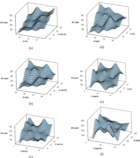
Fig. 3. Interaction effects of process parameters on radial overcut: a) Interaction effects of electrolyte concentration and voltage on radial overcut, b) Interaction effects of electrolyte concentration and initial machining gap on radial overcut, c)

Interaction effects of electrolyte concentration and tool feed rate on radial overcut, d) Interaction effects of voltage and

initial machining gap on radial overcut, e) Interaction effects of voltage and tool feed rate on radial overcut, and f)

185

Voltage (V)

E

le

c

tr

o

ly

te

c

o

n

c

e

n

tr

a

ti

o

n

(

w

t%

)

15 14 13 12 11 10 9 20

19

18

17

16

15

14

> – – – < 200

200 250

250 300

300 350

350 OC (µm)

(a)

Tool feed rate (µm/s)

In

it

ia

l

m

a

c

h

in

in

g

g

a

p

(

µ

m

)

15 14 13 12 11 10 9 8 7 6 80

75

70

65

60

55

50

> – – – < 200

200 250

250 300

300 350

350 O C (µm)

(b)

Fig. 4. Interaction effects of process parameters on radial overcut: a) Interaction effects of electrolyte concentration and voltage on radial overcut, b) Interaction effects of tool feed rate and initial machining gap on radial overcut.

Fig. 5. Back-propagation MLP network [21].

In this study, the back-propagation neural network was used, since it was considered to be a powerful technique for constructing non-linear functions between several inputs and one or more corresponding outputs according to Klimasauskas et al. [22]. While being a relatively simple and flexible tool for data modeling and analysis, it could handle large amounts of data in complex problems.

186 ] [s q

X

=Current output state of the qth neuron in layer

] [s qp q

W = Weight on the connection joining the Pth neuron in layer S-1 to the qth neuron in layer S

] [s q

I

= Weighted summation of inputs to the qth neuron in layer S

A back-propagation element therefore propagates its inputs as:

) ( )

( [ ] [ 1] [ ]

] [ s q p s p s qp s

q f W X f I

X _

       

_

 (2)

where f is a differentiable function, but usually the sigmoid function given by:

1

)

0

.

1

(

)

(

z





e

z 

f

(3)

A global error function E (which is a differentiable function of all the connection weights in the network) is needed to define the local errors at the output layer; so, they can be propagated back through the network. Here, the critical parameter that is passed through the layers is defined by:

) (

)

( [ ] [ 1] [ 1]

] [ ] [       



_

_uq s

u s u s q s q s

q f I e W

I E

e (4)

which can be considered as a measure of the local error for processing element q at level s (here, s+1 is a layer above layer s). The aim of the learning process is to minimize the global error E of the system by modifying the weights. A given set of current weights [s]

qp

W should then be increased or decreased to decrease the global error. This issue can be done by a gradient descent rule as:

] 1 [ ] [ ] [ ] [ 



















_{c q} s _ps

s qp c

s

qp

l

e

X

W

E

l

W

(5) where

l

_c is a learning coefficient. Each weight is to be changed according to the size and direction of negative gradient on the error surface.

In neural network designing process, the optimal structure of neural network (right number of hidden layer as well as right number of neuron in each hidden layer) can be found out by

‘"trial-and-error"’ method only. More layers can give a better fit; but, training takes longer. Too few neurons give a poor fit, while too many neurons result in the over-training of the net.

Electrolyte concentration, voltage, initial machining gap, and tool feed rate are considered as the input variables and radial overcut is the output. Four data sets are selected randomly as the testing data and the remaining twelve data sets are used for specifying the neural networks. In order to have accurate models, several back-propagation MLP neural networks, which are not shown in this section, were used to obtain the best neural network architecture and learning coefficients.

For constructing the model, the tahnaxon transfer function and the momentum (MOM) learning rule were used for training the model. Network with four inputs, nine neurons in the first hidden layer, two neurons in the second hidden layer, and one neuron in output layer, 4:9:2:1, was considered. The related training parameters for the network were optimized as the learning rate=0.7 and maximum number of iteration/epochs=200 for target error of 0.01. The number of weights and biases was 526. It is noticeable that multilayer feed-forward back-propagation is very sensitive to the initial weight assignment. Also, it suffers from a local minima issue. Different estimation results can be obtained even if the network structure and training data are kept constant.

4. 3. Modular neural network (MNN)

187 design the modular topology based on the data.

There are no guarantees that each module is specializing its training on a unique portion of the data. In Fig. 6, an example of modular architecture is given.

Fig. 6. An example of modular architecture [23].

The proposed MNN architecture for predicting radial overcut is as follows:

1.Number of hidden layers = 2

2. Number of upper processing elements in the first hidden layer = 6

3. Number of lower processing elements in the first hidden layer = 5

4. Number of upper processing elements in the second hidden layer = 5

5. Number of lower processing elements in the second hidden layer = 4

6. Transfer function of hidden layers = TanhAxon 7. Learning rule = MOM

8. Momentum value of hidden layers = 0.8 9. Number of output processing elements = 1 10. Transfer function of output layers = TanhAxon 11. Momentum value of output layers = 0.85 12. Learning rate Step size = 1

13. Target error = 0.01

14. Termination criteria = MSE 15. Number of training datasets = 12 16. Number of testing datasets = 4 4. 4. Generalized feed forward (GFF)

Generalized feed forward networks are a generalization of the MLP such that

connections can jump over one or more layers (Fig. 7). In theory, an MLP can solve any problem that a generalized feed forward network can solve. In practice, however, generalized feedforward networks often solve the problem much more efficiently. A classic example is the two spiral problem. Without describing the problem, it suffices to say that a standard MLP requires hundreds of times more training epochs than the generalized feed forward network containing the same number of processing elements.

Fig. 7. Schematic diagram of GFF [24].

For constructing the GFF model, the tahnaxon transfer function and the MOM learning rule were used for training the model. Network with four inputs, seven neurons in the first hidden layer, five neurons in the second hidden layer, and one neuron in the output layer, 4:7:5:1, was considered. The related training parameters for the network were optimized as the learning rate

=0.7 and maximum number of

iteration/epochs=300 for target error of 0.01. The momentum values associated to the hidden and output layers of the network were set to 0.7. 4. 5. Coactive neuro fuzzy inference system (CANFIS)

188

that would combine the benefits of the fuzzy system and neural network. The resulting neuro fuzzy system, a hybrid, has a fuzzy system architecture, but uses neural network learning techniques so that it can be trained automatically. For a given input/output dataset, ANFIS can construct a fuzzy inference system whose membership functions are tuned by either a back-propagation algorithm alone or in combination with the least square method [25].

CANFIS combines some single-output ANFIS models to produce a multiple-output model with nonlinear fuzzy rules which is an advantage of CANFIS model. There are many ways to form a CANFIS from ANFIS, one of which is illustrated in Fig. 8. This diagram is used to maintain the same antecedents of fuzzy rules among multiple ANFIS models. It means that fuzzy rules are constructed with shared membership values to express possible correlations between outputs in this diagram.

Besides, a multiple ANFIS (MANFIS) can be also formed by placing many ANFIS models side by side, in which each ANFIS has an independent set of fuzzy rules [26]. In MANFIS, no modifiable parameters are shared by the juxtaposed ANFIS models. Each ANFIS has an independent set of fuzzy rules, which makes it difficult to realize possible correlations between outputs. Also, the adjustable parameters increase with the increase in the number of outputs [27]. More information about ANFIS, MANFIS, and CANFIS can be found in reference [27].

In neuro fuzzy-based model, the number of input sets is equal to the input variants. For this system, the electrolyte concentration, voltage, initial machining gap, and tool feed rate are the input variations. The model has one output variable with respect to the predicted value of radial overcut. Four data sets are selected randomly as the testing

Fig. 8. Two-output CANFIS architecture with two rules per output [26].

data and the remaining twelve data sets are used for training. A developed CANFIS model used Gaussian membership function (MF) with two MFs per input, MOM learning rule during training process, and TSK fuzzy model proposed by Takagi, Sugeno, and Kang for fuzzy part in these hybrid systems. Network architecture for co-active neuro fuzzy model is as follows:

1. Number of input processing elements = 4 2. Number of membership functions for each input = 2

3. Type of membership functions = Gaussian 4. Number of output processing elements = 1 5. Number of output membership functions = 2 6. Number of hidden layers for output layer = 0 7. Transfer function of output layer = Axon

8. Learning rule = MOM 9. Learning rate step size = 1 10. Target error = 0.01

11. Termination criteria = MSE

12. Maximum epochs for each run = 200 13. Type of fuzzy model = TSK

14. Number of weights and biases = 1893 15. Number of training datasets = 12 16. Number of testing datasets = 4 5. Results and discussion

189 (a)

(b)

(c)

(d)

(e)

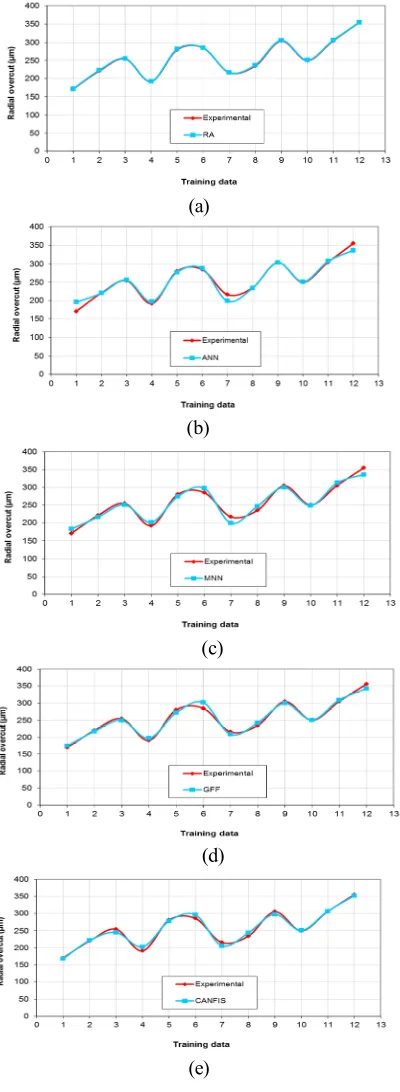
Fig. 9. Comparing the experimental data and predicted radial overcut using the training data for: a) RA, b) MLP, c) MNN, d) GFF, and e) CANFIS.

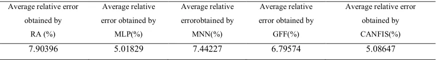
Validation of RA, MLP, MNN, GFF, and CANFIS models was performed using the testing dataset. Testing dataset and predicted values are shown in Table 2. Average relative errors were obtained for RA, MLP, MNN, GFF, and CANFIS, the methodologies were compared, and the results are shown in Table 3. The results illustrated MLP and CANFIS models had much better predicting capability than the other models. Both of the methods were suitable for estimating radial overcut in the acceptable error ranges. But, as a result of the comparative study, it was found that the network based on MLP provided the best results.

6. Conclusions

In this study, RA, MLP, MNN, GFF, and CANFIS models were developed to correlate the input process parameters, such as electrolyte concentration, voltage, initial machining gap, and tool feed rate with the performance measure called radial overcut during the electrochemical drilling of stainless steel material. Using a large number of statistical and soft computing network architecture, CANFIS with Gaussian membership function, TSK fuzzy model, and 4:9:2:1 ANN model were found to be the optimal ones, which can estimate radial overcut with 5.08 and 5.02% overall mean prediction error, respectively. Results showed the potential application of ANN and CANFIS for offline input selection, which could open up the potential use of optimized inputs in machining processes. Based on the 3D surface, contour, and main effect plots, the most dominant parameter for the radial overcut was found as voltage, while the second ranking factor was electrolyte concentration.

References

[1] H. El-Hofy, Advanced machining processes. McGraw-Hill, New York, (2005).

190

Table 2. Testing dataset and predicted values for testing data. Electrolyte

concentration (wt.%)

Voltage (V)

Initial machining gap

(µm)

Tool feed rate (µm /s)

RA MLP MNN GFF CANFIS

14 11 60 9 194.123 198.721 190.585 191.562 198.012 16 9 60 12 191.846 195.869 185.968 188.288 180.352 18 15 60 6 321.792 334.957 325.124 340.0363 334.802 20 11 70 6 299.997 326.277 297.311 302.510 296.284

Table 3. Average relative errors for testing data. Average relative error

obtained by RA (%)

Average relative

error obtained by MLP(%)

Average relative

errorobtained by MNN(%)

Average relative

error obtained by GFF(%)

Average relative error

obtained by CANFIS(%)

7.90396 5.01829 7.44227 6.79574 5.08647

[3] W. Wang, D. Zhu, N. S. Qu, S. F. Huang and X. L. Fang, “Electrochemical drilling with vacuum extraction of electrolyte”, Journal of Materials Processing Technology, Vol. 210, No. 2, pp. 238-244, (2010).

[4] D. Zhu, W. Wang, X. L. Fang, N. S. Qu and Z. Y. Xu, “Electrochemical drilling of multiple holes with electrolyte-extraction”, CIRP Annals - Manufacturing Technology, Vol. 59, No.1, pp. 239-242, (2010).

[5] W. Wang, D. Zhu, N. S. Qu, S. F. Huang and X. L. Fang, “Electrochemical drilling inclined holes using wedged electrodes”, Int. J. Adv. Manuf. Technol., Vol. 47, No. 11, pp. 29-1136, (2010).

[6] Z. W. Fan and L. W. Hourng, “Electrochemical micro-drilling of deep holes by rotational cathode tools”, Int. J. Adv. Manuf. Technol., Vol. 52, No. 5-8, pp. 555-563, (2011).

[7] Z. W. Fan, L. W. Hourng and M. Y. Lin, “Experimental investigation on the influence of electrochemical micro-drilling by short pulsed voltage”, Int. J. Adv. Manuf. Technol., Vol. 61, No. 9-12, pp. 957-966, (2012).

[8] M. A. H. Mithu, G. Fantoni and J. Ciampi, “The effect of high frequency and duty cycle in electrochemical microdrilling”, Int. J. Adv. Manuf.

Technol., Vol. 55, No. 9-12, pp. 921-933, (2011).

[9] H. P. Tsui, Hung, J. C. You and B. H. Yan, “Improvement of electrochemical microdrilling accuracy using helical tool”, Materials and Manufacturing Processes, Vol. 23, No. 5, pp. 499-505, (2008).

[10] Y. Liu and S. F. Huang, “Experimental Study on Electrochemical Drilling of Micro Holes with High Aspect Ratio”, Advanced Materials Research, Vol. 941-944, pp. 1952-1955, (2014).

[11] S. Zare Chavoshi, “Analysis and predictive modeling of performance parameters in electrochemical drilling process”, Int. J. Adv. Manuf. Technol., Vol. 53, No. 9-12, pp. 1081-1101, (2011).

[12] S. Zare Chavoshi and M. Tajdari, “Surface roughness modelling in hard turning operation of AISI 4140 using CBN cutting tool”, Int. J. Mater Form, Vol. 3, No. 4, pp. 233-239, (2010). [13] M. R. Soleymani Yazdi and S. Zare

Chavoshi, “Analysis and estimation of state variables in CNC face milling of AL6061”, Prod. Eng. Res. Devel., Vol. 4, No. 6, pp. 535-543, (2010).

191 Manuf., Vol. 19, No. 4, pp. 473-483,

(2008).

[15] B. R. Sarkar, B. Doloi and B. Bhattacharyya, “Parametric analysis on electrochemical discharge machining of silicon nitride ceramics”, Int. J. Adv. Manuf. Technol., Vol. 28, No. 9-10, pp. 873-881, (2006).

[16] D. S. Bilgi et al, “Predicting radial overcut in deep holes drilled by shaped tube electrochemical machining”, Int. J. Adv. Manuf .Technol., Vol. 39, No. 1-2, pp. 47-54, (2008).

[17] Z. Uros, C. Frank and K. Edi, “Adaptive network based inference system for estimation of flank wear in end-milling”, Journal of materials processing technology, Vol. 209, No. 3, pp. 1504-1511, (2009).

[18] U. Caydas, A. Hascalik and S. Ekici, “An adaptive neuro-fuzzy inference system (ANFIS) model for wire-EDM”, Expert Systems with Applications, Vol. 36, No. 3, pp. 6135-6139, (2009).

[19] J. Antony, “Design of Experiments for Engineers and Scientists”, Elsevier Science & Technology Books, ISBN: 0750647094, (2003).

[20] R. Venkata Rao, “Advanced Modeling and Optimization of Manufacturing Processes”, Springer, (2011).

[21] M. S. Chen, “Analysis and design of the multi-layer perceptron using polynomial

basis functions”, Doctor of philosophy thesis, The University of Texas at Arlington, (1991).

[22] C. C. Klimasauskas, “Neural Computing. Neural- Ware”,Pittsburgh, (1991). [23] A. Schmidt, “A modular neural network

architecture with additional

generalization abilities for high dimensional input vectors”, Master of Science thesis, Manchester Metropolitan University, (1996).

[24] K. B. Khanchandani and M. A. Hussain, “Emotion recognition using multilayer perceptron and generalized feed forward neural network”, Journal of scientific and industrial research, Vol. 68, pp. 367-371, (2009).

[25] X. Li, X. Guan, Y. Li and A. Hybrid, “Radial Basis Function Neural Network for Dimensional Error Prediction in End Milling”, ISNN 2004, LNCS 3174, pp. 743-748, (2004).

[26] N. Q. Dinh and N. V. Afzulpurkar, “Neuro-fuzzy MIMO nonlinear control for ceramic roller kiln”, Simulation Modelling Practice and Theory, Vol. 15, No. 10, pp. 1239-1258, (2007).