www.geosci-model-dev.net/9/1891/2016/ doi:10.5194/gmd-9-1891-2016
© Author(s) 2016. CC Attribution 3.0 License.
An optimized treatment for algorithmic differentiation of an
important glaciological fixed-point problem
Daniel N. Goldberg1, Sri Hari Krishna Narayanan2, Laurent Hascoet3, and Jean Utke4 1Univ. of Edinburgh, School of GeoSciences, Edinburgh, UK
2Maths. and Comp. Science Division, Argonne National Lab, Argonne, IL, USA 3INRIA Sophia-Antipolis, Valbonne, France
4Allstate Insurance Company, Northbrook, IL, USA
Correspondence to: Daniel N. Goldberg ([email protected])
Received: 14 January 2016 – Published in Geosci. Model Dev. Discuss.: 3 February 2016 Revised: 22 April 2016 – Accepted: 27 April 2016 – Published: 20 May 2016
Abstract. We apply an optimized method to the adjoint gen-eration of a time-evolving land ice model through algorith-mic differentiation (AD). The optimization involves a spe-cial treatment of the fixed-point iteration required to solve the nonlinear stress balance, which differs from a straight-forward application of AD software, and leads to smaller memory requirements and in some cases shorter computa-tion times of the adjoint. The optimizacomputa-tion is done via im-plementation of the algorithm of Christianson (1994) for re-verse accumulation of fixed-point problems, with the AD tool OpenAD. For test problems, the optimized adjoint is shown to have far lower memory requirements, potentially enabling larger problem sizes on memory-limited machines. In the case of the land ice model, implementation of the al-gorithm allows further optimization by having the adjoint model solve a sequence of linear systems with identical (as opposed to varying) matrices, greatly improving perfor-mance. The methods introduced here will be of value to other efforts applying AD tools to ice models, particularly ones which solve a hybrid shallow ice/shallow shelf approxima-tion to the Stokes equaapproxima-tions.
1 Introduction
In recent decades it has become clear how little we un-derstand about the processes governing ice sheet behavior (Vaughan and Arthern, 2007), and the complexity that is re-quired in numerical ice sheet models in order to understand this behavior (Little et al., 2007; Lipscomb et al., 2009). The
representation of poorly understood processes in ice sheet models leads to large, poorly constrained parameter sets, the size of which might potentially scale with the size of the numerical grid. It is vital that there be a means to relate the output of an ice sheet model back to these parameters, both comprehensively and efficiently. However, the simplest method of sensitivity assessment – running the model multi-ple times while varying each parameter in isolation – quickly becomes intractable because of the complexity of the mod-els. Consider, for instance, a dynamic model of the Antarctic Ice Sheet, which takes several days to run on a supercomput-ing cluster, and contains several hundred thousand parame-ters pertaining to the spatially varying frictional and geother-mal properties of the bed over which it slides. Assessing the sensitivity of the model to this parameter field by the method described above would not be feasible.
Adjoint models provide a means to assess these sensitivi-ties in a way which is independent of the number of param-eters. The adjoint of an ice sheet model simultaneously cal-culates the derivatives of a single model output (often called a “cost function”) with respect to all model parameters – or rather, the gradient of the cost function with respect to the parameter set, or control variables. Note that the latter com-putation more naturally lends itself to scientific inquiry, as
– an investigator is unlikely to solely be interested in just one of these (potentially) several hundred thousand poorly constrained parameters.
The adjoint model is essentially the linearization of the model, only the information is propagated backward in time (or rather in reverse to computational order). As such, the original model is often referred to as the “forward model”. Essentially, it is this backward-in-time propagation that al-lows for simultaneous calculation of these derivatives, re-gardless of the dimension of the parameter set.
One of the earliest instances of the use of the adjoint of an ice sheet flow model was that of MacAyeal (1992), in which a control method was developed to optimally fit a model to observed velocities through adjustment of bed friction pa-rameters. The ice flow model used in this study was a depth-integrated approximation to the shear-thinning Stokes equa-tions, appropriate to ice shelves and weak-bedded streams (MacAyeal, 1989). Moreover, it was a static model, i.e., it consisted only of the nonlinear stress balance governing ice velocities, and did not evolve the ice geometry or temper-ature. The method has since been used in a number of ap-plications (e.g., MacAyeal et al., 1995; Rommelaere, 1997; Vieli and Payne, 2003; Larour et al., 2005; Khazendar et al., 2007; Sergienko et al., 2008; Joughin et al., 2009). Similar methods have been applied to higher-order approximations (Pattyn et al., 2008), or to the Stokes equations themselves (e.g., Morlighem et al., 2010; Goldberg and Sergienko, 2011; Petra et al., 2012; Perego et al., 2014; Isaac et al., 2015).
More recently, algorithmic differentiation (AD) tools have been applied to ice sheet models for adjoint model genera-tion. AD tools differentiate models by applying the chain rule to their numerical values (e.g., Forth et al., 2012; Naumann, 2012, also see www.autodiff.org). They have been applied extensively to atmospheric and ocean codes (Errico, 1997; Heimbach et al., 2002; Heimbach, 2008). The use of AD of-fers ease of differentiation of the model. For instance, the ma-jority of the adjoint models mentioned in the previous para-graph ignore the dependence of nonlinear ice viscosity on strain rates, producing an approximate set of adjoint equa-tions which have the same form as the forward model, al-lowing for code reuse. At the same time, this approximate adjoint ignores terms in the model gradient without know-ing whether they are negligible. While the full adjoint model involves equations distinct from the forward model, the use of AD avoids having to write the code to solve them. An-other advantage is modularity. Modifying, for example, the specific form of strain-rate dependence of viscosity in an ice sheet model would then require invasive changes to an an-alytically derived set of adjoint equations. When generating the adjoint through AD, these changes are automatic. Fur-thermore, AD tools are invaluable when dealing with time-dependent or multiphysics models, where model complexity makes it very difficult to generate adjoint code by hand. In fact, to date the only time-dependent ice sheet adjoint
mod-els have been generated through the use of AD (Heimbach and Bugnion, 2009; McGovern et al., 2013; Goldberg and Heimbach, 2013; Larour et al., 2014).
For clarity, we will draw a distinction between the partial differential equations (PDEs) that comprise a mathematical model of a physical system, and the computational model that discretizes these equations. The PDEs represent an oper-ator, the linearization of which has an adjoint (the continuous adjoint), which can be discretized (Goldberg and Sergienko, 2011). Alternatively, the computational model can be differ-entiated directly. We focus on this discrete adjoint in this paper. As mentioned above, a discrete adjoint model can be thought of as the reverse-order computation of the orig-inal model (Griewank and Walther, 2008; Heimbach and Bugnion, 2009), but an important subtlety is that this discrete adjoint may not necessarily correspond to a discretization of the correct adjoint, a subtlety which bears on the accuracy of ice sheet adjoint models.
Most ice flow models solve a nonlinear elliptic system of (PDEs) for ice velocity, and these equations require an it-erative fixed-point approach. (Here “most ice flow models” is taken to mean “all ice flow models”, except those which make the Shallow Ice Approximation (SIA, Hutter, 1983). The SIA strictly applies only to slow-moving ice frozen at its base, and not the fast-flowing ice streams at the Antarctic and Greenland margin which currently exhibit variability.) We re-fer to this fixed-point iteration as the forward fixed-point iter-ation (FFPI). Ice sheet models of this type, to which AD tools have been applied previously, simply step backward through the FFPI (Goldberg and Heimbach, 2013; Larour et al., 2014; Martin and Monnier, 2014). This strategy is sometimes re-ferred to as the “mechanical adjoint” (Griewank and Walther, 2008). The mechanical adjoint of a fixed-point solution is in fact the iterative solution of a distinct fixed-point prob-lem, whose convergence differs from that of the forward loop (Gilbert, 1992; Christianson, 1994), and to which we refer as the adjoint fixed-point iteration (AFPI). As such, the me-chanical adjoint could potentially perform too many itera-tions, thereby wasting resources; or too few iteraitera-tions, re-sulting in decreased accuracy. In fact, in some cases the me-chanical adjoint can be inaccurate regardless, as we show in Sect. 4.1. Additionally, the mechanical adjoint can lead to burdensome memory and/or recomputation loads as dis-cussed in Sect. 3. Martin and Monnier (2014) show accuracy can be maintained by truncating the iteration in the mechani-cal adjoint, but do not provide a robust, situation-independent way of doing so.
the forward model. Additionally, the equations must poten-tially be re-derived if the model physics are changed. More-over, not all such approximations to the Stokes balance al-low such an approach. Hybrid stress balances, which solve two-dimensional approximations to the Stokes balance and are appropriate for both fast-sliding and slow-creeping flow, are increasing in popularity due to low computational cost but reasonable agreement with the first-order approximation (e.g., Goldberg, 2011; Schoof and Hindmarsh, 2010; Corn-ford et al., 2013; Arthern et al., 2015; W. Lipscomb, personal communication, 2015). Our ice model implements such a hybrid stress balance. Differentiating such a balance at the equation level is possible but very tedious, and leads to very complicated expressions that depend strongly on discretiza-tion (Goldberg and Sergienko, 2011), both undesirable prop-erties.
Christianson (1994) provides a mathematical strategy for finding the adjoint of a fixed-point problem via direct solu-tion of a related fixed-point problem. The convergence of this related problem can be directly evaluated, avoiding the prob-lem of too many or two few iterations. A novelty of the ap-proach is that only information from the converged state of the forward loop is used for the adjoint computation, permit-ting additional efficiency gains. In this paper, we present an application of the AD software OpenAD (Utke et al., 2008) to the MITgcm time-dependent glacial flow model (Goldberg and Heimbach, 2013). A different AD tool has previously been applied to this ice model, so here we focus on the imple-mentation of the Christianson algorithm (henceforth called BC94) – an innovation which is observed to yield substantial improvements in performance.
2 Fixed-point problem
The forward model to which AD methods are applied is that of Goldberg (2011), which is a hybrid of two low-order ap-proximations to the nonlinear Stokes flow equations that gov-ern ice creep over timescales longer than a day (Greve and Blatter, 2009). These are the Shallow Ice Approximation, ap-propriate for slow-flowing ice governed by vertical shear de-formation, and the Shallow Shelf Approximation (SSA; Mor-land, 1987; MacAyeal, 1989), appropriate for fast-flowing ice governed by horizontal stretching and shear deforma-tion. The hybrid equations have been shown appropriate in both regimes, and represent considerable computational sav-ings over the Blatter–Pattyn equations (Blatter, 1995; Pattyn, 2003; Greve and Blatter, 2009), as they require the solution of a two-dimensional system of elliptic PDEs rather than a three-dimensional one.
We do not discuss the details of the model here, as they are given in detail in Goldberg (2011) and in Goldberg and Heimbach (2013). Rather, we focus on its FFPI. Conceptu-ally, the model algorithm can be divided into two compo-nents: prognostic (time dependent) and diagnostic (time
in-dependent). In the MITgcm land ice model, the prognostic component comprises an update to ice vertical thickness (H) through a depth-integrated continuity equation, as well as an update of the surface elevation and, implicitly, the portion of the model domain where ice is floating in the ocean rather than in contact with its bed. The diagnostic component solves the FFPI for ice velocities based on the current thickness pro-file. Mathematically this step can be understood as the inver-sion of a nonlinear operatorF to obtainu:
F (u,a)=f. (1)
Hereuis a vector representing horizontal depth-averaged ve-locitiesuandv.F is the discretization of a nonlinear elliptic PDE in depth-averaged velocity.arepresents the set of ma-terial parameters that determine the coefficients of the PDE: ice thickness (H), basal friction rheological parameters (C), and ice rheological parameters (A).f is the discretization of driving stress (Cuffey and Paterson, 2010), or the depth-integrated hydrostatic pressure gradient (which is determined by ice thickness). In this model (and in many others) the non-linear elliptic equation is solved by a sequence of solutions of linear elliptic operators, where the operators depend on the result of the previous linear solve:
u(m+1)=(L{u(m),a})−1f ≡8(u(m),aˆ), (2)
where, in the definition of8,aˆ represents the augmentation of the setato includef.Lis a linear operator constructed using u(m), the current iterate of u, and the parameters a.ˆ
Note thataˆ will differ for each time step through the depen-dence on ice thickness, which is updated by the prognostic component of the model. In general, the ice rheological pa-rameters depend on ice temperature, which is advected and diffused over time. Our ice model does not have a thermo-mechanical component, but once developed, it will not affect the algorithm we present in this paper.
Equation (2) is our FFPI mentioned previously. In prac-tice, the iteration is truncated when subsequent iterates agree in some predefined sense, but in theory will converge to a unique solutionu∗(aˆ). In the process of computing the ad-joint to the ice model, ∂u∗
∂aˆ must be found, either directly or indirectly. The focus of this paper is an efficient, scalable method of computing this object.
3 Forward model and mechanical adjoint
FOR n = initialTimeStep TO finalTimeStep
// ConstructsaˆfromH[n]:
CALL CALC_DRIVING_STRESS(H[n] ) m = 0
REPEAT UNTIL CONVERGENCE OF u
u = Φ(u,ˆa) m = m+1
store L, u and other variables
lastm[n] = m
// FindsH[n+1]from continuity equation with
u: CALL ADVECT_THICKNESS()
Pseudocode 1. Pseudocode version of forward model time-stepping procedure.
parameters; then the prognostic component updates thick-ness (ADVECT_THICKNESS). The function 8 comprises the construction of the linear systemL (including the non-linear dependence of the matrix coefficients on the previous iterate) and its solution.
Pseudocode 2 gives an overview of our implementation of the mechanical adjoint. Here we introduce some nota-tion: for a given computational variable X, the adjoint to X, which formally belongs to the dual tangent space atX, is denoted δ∗X (e.g., Heimbach and Bugnion, 2009; see also Bartholomew-Biggs et al., 2000; Griewank and Walther, 2008). The algorithm evolves the adjoint variables (e.g., δ∗H) backward in time. These adjoint variables carry with them the sensitivities of the model output to the correspond-ing forward variables, and the sensitivities are eventually propagated back to the input parameters. Note that the ad-joints of the individual (pseudo) subroutines are given and correspond to the (pseudo) subroutines of the forward model, mirroring the way the adjoint is actually constructed. Just like the forward model, the adjoint contains an inner loop – this is a specific implementation of the AFPI, which will be discussed in further detail below. As the computation of 8involves the solution of a linear system of equations, the adjoint of8involves the solution of the adjoint of that sys-tem. Since the matrix L{u(m),a}is self adjoint, it is easier
to calculate this result analytically than for an AD tool to differentiate the linear solver code (e.g., Goldberg and He-imbach, 2013). This allows for invocation of external black box libraries that cannot be differentiated by the tool. This analytical approach allows invocation of AD for ice models (e.g., Martin and Monnier, 2014).
An important point to be made is that the inner loop in Pseudocode 2 is executed as many times as the correspond-ing inner loop in the forward model (lastm[n]), without any checks of convergence. This could lead to under- or overcon-vergence, as stated previously. Another important aspect is
FOR n = finalTimeStep DOWNTO initialTimeStep
// Constructsδ∗H[n]andδ∗u[n]fromδ∗H[n+1] // via the adjoint of the continuity equation :
CALL AD_ADVECT_THICKNESS()
REPEAT lastm[n] TIMES
restore L, u and other variables
δ∗aˆ = δ∗aˆ+δ∗u ∂Φ ∂aˆ T
δ∗u = δ∗u ∂Φ ∂u
T
// Updatesδ∗H[n]fromδ∗aˆ:
CALL AD_CALC_DRIVING_STRESS(δ∗H[n])
Pseudocode 2. Pseudocode version of mechanical adjoint.
that at each reverse time step, and, importantly, at each itera-tion of the FFPI, the state of the forward model is required. In particular, every matrixL{u(m),a}must be stored (or
recom-puted), along with other intermediate variables within the fixed-point loop. The storage and recovery steps are shown explicitly in Pseudocodes 1 and 2 – and can lead to burden-some memory loads depending on the number of fixed-point iterations taken at each time step.
The mechanical adjoint of our model was first generated using TAF (Transformation of Algorithms in Fortran; Gier-ing et al., 2005), but has subsequently been generated via OpenAD with little further difficulty.
4 Fixed-point treatment
Christianson (1994) presents an algorithm (BC94) for calcu-lating the adjoint of a fixed-point problem that addresses the shortcomings given above, namely the dependence of the ter-mination of the adjoint loop on that of the forward loop, and the requirement to store variables at each iteration of the ad-joint loop. Additionally, it provides the opportunity for fur-ther optimization when applied to a higher-order ice sheet model, as discussed below.
4.1 Mathematical basis
For a rigorous mathematical analysis of BC94, the user is asked to consult the original paper. Here, we give a brief overview of its mathematical basis. In terms of Eq. (2), con-sider the converged state of the fixed-point problem:
u∗=8(u∗,aˆ). (3)
Consider a total differential of this equation: δu∗=
∂8
∂u(u∗,aˆ)δu∗+ ∂8
∂aˆ (u∗,aˆ)δaˆ. (4) Rearranging gives
δu∗=
I−∂8 ∂u
−1∂8
If the operator norm of the square matrix∂8/∂uis less than unity then the above is equivalent to
δu∗=
I+∂8/∂u+(∂8/∂u)2
+(∂8/∂u)3+. . .∂8
∂aˆδaˆ. (6)
Note that in the above series,∂8/∂uis always evaluated at the converged solutionu∗. The above condition on the norm of∂8/∂uwill not hold in general – but since this is one of the conditions required to ensure convergence of8to a fixed point, we can expect that it will be satisfied atu∗.
From Eq. (6) we obtain the desired adjoint operator, ap-proximated by a truncated series of lengthn:
δ∗aˆ=
∂8 ∂aˆ
T
I+
∂8 ∂u
T
+
∂8 ∂u
T!2
+. . .
+
∂8
∂u
T!n#
δ∗u∗. (7)
The algorithm of Christianson (1994) essentially con-structs the operator within brackets in Eq. (7) via a fixed-point loop, the convergence criterion of which determines the truncation length n. This loop represents an implemen-tation of the AFPI, distinct from the one implemented by the mechanical adjoint. In order to make this distinction explicit, the operator in Eq. (7) can be written
n X
i=0
∂8 ∂aˆ
T n
Y
k=n+1−i
∂8 ∂u
T
, (8)
where it is understood that in thei=0 term the product se-quence evaluates to the identity. It is straightforward to check that the mechanical adjoint (cf. Pseudocode 2) effectively computes the operator
n X
i=0
∂8(n−i) ∂aˆ
T n
Y
k=n+1−i
∂8(k) ∂u
T
, (9)
where∂8(k)/∂uand similar terms indicate that the gradient
is calculated using the variables that have been stored at for-ward iteration k, rather than at the converged solution. It is apparent that this expression can differ from Eq. (7) if some iterates are far from the fixed point, or if the gradient of8is sensitive tou. In fact, it has been observed in certain cases that a poor choice of initial iterate can lead to inaccurate ad-joint calculation. Furthermore, in the mechanical adad-joint, the truncation length depends on the number of forward itera-tions, which may not be related to the convergence of this se-ries. A scheme which truncates this series based on the size of the truncated terms will be more robust.
4.2 Implementation in OpenAD
Pseudocodes 3 and 4 give an overview of our implemen-tation of BC94 in the MITgcm ice model using OpenAD.
FOR n = initialTimeStep TO finalTimeStep
// ConstructsaˆfromH[n]:
CALL CALC_DRIVING_STRESS(H[n] )
u = initial guess
CALL PHISTAGE(PRELOOP, w, u, ˆa)
REPEAT UNTIL CONVERGENCE OF u
CALL PHISTAGE(INLOOP, w, u, aˆ)
CALL PHISTAGE(POSTLOOP, w, u, aˆ)
// FindsH[n+1]from continuity equation withu: CALL ADVECT_THICKNESS()
SUBROUTINE PHISTAGE(phase, w, u, aˆ)
IF (phase==PRELOOP)
// do nothing
ELSE IF (phase==INLOOP)
save tape pointer
u = Φ(u,aˆ)
// Makes sure no storage is done : restore tape pointer
ELSE IF (phase==POSTLOOP)
u = Φ(u,aˆ)
store L, u and other variables
Pseudocode 3. Pseudocode version of modified forward model for BC94.
High-level changes to the code were necessary, but the sub-routines that comprise the action of the operator8were left unchanged. As shown in Pseudocode 3, rather than calling 8directly, the loop implementing the FFPI calls a subrou-tine calledPHISTAGEwith an argumentphasewhich has valuesPRELOOP,INLOOP, orPOSTLOOP. Just before the fixed-point loopPHISTAGEis called withPRELOOP, which does nothing (that is, nothing in forward mode). Within the loop,PHISTAGEis called with argument INLOOP, which essentially has the same effect as the call to8in the orig-inal ice model time-stepping algorithm. After the loop is converged,PHISTAGEis called with argumentPOSTLOOP, which calls8one more time (which, if the iteration is con-verged, should have negligible effect). Of key importance is that any storing of variables that takes place within the call to8in theINLOOPphase is undone at the end of each it-eration. Once convergence is reached, storing takes place as normal in thePOSTLOOPphase.
sim-FOR n = finalTimeStep DOWNTO initialTimeStep
// Constructsδ∗H[n]andδ∗ufromδ∗H[n+1] // via the adjoint of the continuity equation : CALL AD_ADVECT_THICKNESS()
CALL AD_PHISTAGE(POSTLOOP, δ∗w, δ∗u, δ∗ˆa)
REPEAT UNTIL CONVERGENCE OF δ∗w
CALL AD_PHISTAGE(INLOOP, δ∗w, δ∗u, δ∗aˆ) CALL AD_PHISTAGE(PRELOOP, δ∗w, δ∗u, δ∗aˆ)
δ∗u = 0.0 // Updatesδ∗H[n]
fromδ∗ˆa:
CALL AD_CALC_DRIVING_STRESS(δ∗H[n])
SUBROUTINE AD_PHISTAGE(phase, δ∗w, δ∗u, δ∗aˆ) IF (phase==POSTLOOP)
δ∗w = δ∗u
ELSE IF (phase==INLOOP)
save tape pointer
restore L, u and other variables
δ∗w = δ∗w ∂Φ ∂u
T +δ∗u
// Makes sure converged state is reused : restore tape pointer
ELSE IF (phase==PRELOOP)
δ∗aˆ = δ∗w ∂Φ ∂ˆa
T
Pseudocode 4. Pseudocode version of fixed-point (BC94) adjoint.
plest to apply the template mechanism provided by OpenAD, that lets the end-user provide a customized differentiation of specific sections of the code by means of a template, hand-written once and for all. Such a template was hand-written for
PHISTAGEin order to implement the pseudocode in Pseu-docodes 3 and 4. The subroutine thus serves as a layer which does not affect the diagnostic ice physics represented by the function8or the prognostic physics implemented outside of the FFPI loop. Thus, the modularity offered by the AD ap-proach is not lost.
Pseudocode 4 shows how the adjoint model is constructed, making use of the OpenAD-generated adjoint code for 8. In adjoint mode, the calls toPHISTAGEhappen in reverse order. The variable w is a placeholder with no real role in the forward computation, but the adjoint of the call to
PHISTAGEin thePOSTLOOPphase assigns toδ∗wthe ad-joint of velocity resulting fromAD_ADVECT_THICKNESS, in other wordsδ∗u∗. In theINLOOPphase,δ∗wis updated according to the equation
δ∗w(m+1)=δ∗w(m)
∂8
∂u
T
+δ∗u, (10) wheremindicates the AFPI iteration step. (In the table the subscript indices are left off for clarity). This assignment is equivalent to step 9 of Algorithm 9.1 of Christianson (1994).
Given that δ∗w is initialized to δ∗u∗, it can be seen that δ∗w(n) is equivalent to the argument of ∂8∂aˆ
T
in Eq. (7). Christianson (1994) observes furthermore that if the conver-gence criteria are met, any other initialδ∗w(0)will converge
toδ∗aˆfor a sufficientn. This property can be used to imple-ment a warm start of the algorithm when a good initial guess ofδ∗wis available. We did not test this idea for our present experiments. Finally, the adjoint-mode call toPHISTAGE
withPRELOOPrepresents the operation of ∂8
∂aˆ
T
on the re-sult.
The introduction of the variablewrepresents the bulk of the modifications that were necessary to implement the al-gorithm using OpenAD. The only additional modification is a handwritten evaluation of convergence ofδ∗w: we termi-nate when the relative reduction in the norm of the change in δ∗w is below a fixed tolerance. The norm in which conver-gence is evaluated is the conjugate norm to that used in the forward iteration: that is, if forward convergence is evaluated in theLpnorm, then adjoint convergence is evaluated in the Lqnorm, where p1+1q=1 (and theL1norm is conjugate to the sup norm). Though all norms are equivalent in a finite-dimensional vector space, this feature is added for complete-ness, motivated by the fact that the error in the derivative is bounded by the inner product of the error in the forward it-eration and the error in the reverse itit-eration (Christianson, 1998). In the results presented in this paper, convergence of the forward iteration is evaluated in the sup norm (thus ad-joint convergence is evaluated in theL1norm).
We emphasize that all of these modifications are at the level of the wrapperPHISTAGE, which does not contain any representation of model physics (and hence changes to the model physics would not require changes to this subroutine nor to its adjoint template).
4.3 Optimization of linear solver
As mentioned previously, evaluating8involves the solution of a large (self-adjoint) linear system, and thus the adjoint of8involves the solution of a linear system with the same matrix (assuming the same values ofu anda). In the me-ˆ chanical adjoint model, within a given time step, this matrix differs with each iteration of the adjoint loop; however, in BC94, only the right-hand side differs. This invariance sug-gests the use of a linear solver whose cost can be amortized over a number of solves, such as an LU decomposition or an algebraic multigrid preconditioner, the internal data struc-tures of which only need be constructed once. In this study, we consider only an LU solver.
5 Test experiment
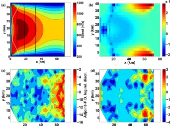
advanc-Figure 1. (a) Surface speed (shading) in the test experiment. The flow direction is from right to left, and the white portion of the figure is where the ice shelf has not advanced to the end of the domain. Black contours give thickness spaced every 200 m and the white contour is the grounding line. (b) Adjoint sensitivities of ice speed to basal melt rates. (c) The (log) relative discrepancy between adjoint sensitivities and the gradient calculated via finite differencing. (d) The (log) second-order differencing of cost functionJ(see Eq. 17).
ing ice stream and shelf in a rectangular domain (x, y)∈ [0,80 km] × [0,40 km]. We prescribe an idealized bedrock topographyRand initial thicknessh0.Rdoes not vary in the along-flow (x) direction and forms a channel through which the ice flows, prescribed by
R(x, y)= −600−300×sin πy 40 km
, (11)
while initial thickness is given by
h0(x, y)=
300 m+min
1,x−62 km50 km 2
×1000 m 0≤x <50 km
300 m 50 km≤x≤70 km.
(12)
Where x >70 km, there is open ocean (until the ice shelf front advances past this point). Where ice is grounded, a lin-ear sliding governs basal stress:
τb= −Cu, (13)
whereC=25 Pa (a−1m). The Glen’s law coefficient (which controls the ice stiffness) is given by 8.5×10⁻¹⁸Pa−3a−1, corresponding to ice with a uniform temperature of ∼ −34◦C. At the upstream boundary, ice flows into the do-main at x=0 at a constant volume flux per meter width of 1.5×10⁶m2a−1. Aty=0 andy=40 km no-flow conditions
are applied. Velocity, thickness, and grounding line are plot-ted in Fig. 1a. Further details of the equations are given in Goldberg and Heimbach (2013).
In the experiment, a cost functionJ is defined by running the model forward in time for 8 years, and evaluating the summed square velocity at the end of the run. That is, J=X
i,j
u(i, j )2+v(i, j )2, (14) whereiandj indicate cell indices in thex andydirections, respectively, and u andv are cell-centered surface veloci-ties. Unless specified otherwise, the time step is 0.2 years and grid resolution is 2000 m, so 1≤i≤40 and 1≤j ≤20. The control variable consists of basal melt ratem, defined for each cell and considered constant over a cell and in time (and nonzero only where ice is floating), and set uniformly to zero in the forward run, even under floating ice (in real-ity, there would be background melting to be perturbed, and changes to these melt rates would elicit responses of similar magnitudes, but background melting is zero for the sake of simplicity). Figure 1b plots the adjoint sensitivities ofm, or alternatively∂J /∂mij, wheremij is melt rate in cell(i, j ).
thickness, and so in the center of the shelf, thinning leads to deceleration. Meanwhile, ice shelf velocities are very insen-sitive to melting at the center of the ice shelf front.
We find that the results of the mechanical adjoint and of the adjoint model implementing BC94 (which we henceforth refer to as the “fixed-point adjoint”) are almost identical, with a relative difference no larger than 10−6 over the do-main (not shown). However, the adjoint sensitivities should also be compared against a direct computation of the gradi-ent, i.e., one which does not involve the adjoint model. In this case∂J /∂mij is approximated through finite
differenc-ing, by perturbing mij by a finite amount and running the
forward model again. This calculation is carried out for each cell (i, j). Figure 1c plots discfd, given by
discfd=
δ∗mfpij−δ∗mcdij δ∗mfp
ij
, (15)
whereδ∗mfpij is obtained through the BC94 algorithm, while δ∗mcdij is a centered-difference approximation:
δ∗mcdij = 1
2(J (mij+)−J (mij−)), (16) andJ (mij+)indicates that the melt rate at cell(i, j )only
is perturbed by.is set to 0.01 m a−1uniformly.
discfdis seen to become quite large, on the order of∼1 % in some parts of the domain, warranting further examination. An implicit assumption in the discrepancy measure discfdis that the finite difference approximation has negligible error, which may not be the case. We can estimate where this finite-difference error will be large: from a Taylor series expansion, and ignoring round-off error (which we do not attempt to estimate), the error in approximating the adjoint sensitivity of mij by finite difference is roughly proportional to the second
derivative∂2J /∂(mij)2. As a proxy for this quantity we plot
in Fig. 1d the second-order difference ofJ:
12Jij=J (mij+)+J (mij−)−2J. (17)
This measure appears to correlate well with discfd, aside from the central part of the ice shelf front. Here, the large relative errors are likely due to the small magnitude of the adjoint sensitivities. We emphasize that Eq. (17) is not an accurate measure of the second derivative – which is obvi-ously not achievable through finite differencing if first-order derivatives are inaccurate – but is simply meant to give an indication of its magnitude.
5.1 Truncation errors
The analysis of Christianson (1994) suggests the error of the calculated adjoint depends linearly on both the reverse trun-cation error and the forward truntrun-cation error. The reverse truncation error is the difference between the final and penul-timate iterates in the adjoint loop, i.e., the error associated
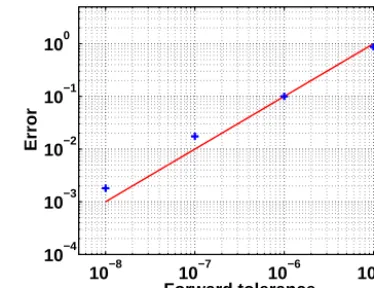
10−8 10−7 10−6 10−5 10−4
10−3 10−2 10−1 100
Forward tolerance
Error
Figure 2. Maximum error in fixed-point adjoint calculation versus tolerance of forward loop. The red line indicates linear dependence.
with terminating the loop after a finite number of iterations. That is, referring to Pseudocode 4, ifmiterations are carried out, the reverse truncation error is equal to
αkwm−wm−1k, (18)
whereαis related to the gradient of8at the fixed point. The norm here is the sup norm, because this is the norm on which our convergence criterion is based.
While a tight bound forαwill vary with each time step, it can be expected that the reverse truncation error will vary linearly with the convergence tolerance and we do not ad-dress it further. However, we investigate the dependence on forward truncation error as follows. A sequence of adjoint model runs is carried out with increasingly smaller toler-ances (from 10−5to 10−8) for the forward fixed-point itera-tion loop. The tolerance of the reverse loop is kept at a small value (10−8). The adjoint sensitivities corresponding to the smallest forward tolerance (10−9) are assumed to be truth; error is estimated by comparison with these values. Figure 2 plots the maximum pointwise error in the adjoint calculation over the domain against the forward tolerance, which is a good measure of the forward truncation error. Within a range of forward truncation error the dependence is nearly linear, although this dependence appears to become weaker as for-ward truncation error becomes smaller.
5.2 Performance
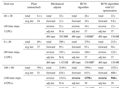
Table 1. Timing performance and memory usage of mechanical and fixed-point adjoints. In the “Plain” column, “avg iter” indicates the number of nonlinear iterations per time step. In other columns, “adj iter” indicates the total number of iterations of the adjoint loop described by Pseudocode 4 divided by the number of time steps. “dbl tape” indicates the length of the double tape. The asterisk indicates that this value falls anywhere between 8 and 136 MB. The highlighted text shows the memory gains of the fixed-point adjoint (bold font) and the performance gain of the fixed-point adjoint (italic font).
Grid size Plain Mechanical BC94 BC94 algorithm (untouched) adjoint algorithm with LU
optimization
40×20 total 6.1 s total 32 s total 26 s total 22 s
avg iter 34 forward 11 s forward 10 s forward 9.8 s
(40 time steps, reverse 21 s reverse 16 s reverse 12 s
1 CPU) adj iter N/A adj iter 37 adj iter 37
dbl tape 392 MB dbl tape 136MB∗ dbl tape 136 MB∗
0×40 total 69 s total 289 s total 278 s total 215 s
avg iter 37 forward 95 s forward 93 s forward 94 s
(80 time steps, reverse 193 s reverse 184 s reverse 122 s
1 CPU) adj iter N/A adj iter 37 adj iter 37
dbl tape 1.42 GB dbl tape 136 MB∗ dbl tape 136 MB∗
160×80 total 591 s total 2149 s total 1994 s total 1553 s
avg iter 51 forward 634 s forward 615 s forward 608 s
(160 time steps, reverse 1514 s reverse 1378 s reverse 944 s
4 CPUs) adj iter N/A adj iter 39 adj iter 39
dbl tape 2.95 GB dbl tape 136 MB∗ dbl tape 136 MB∗
general, keeping the entire trajectory (including intermediate variables) of a time-dependent model run in memory is not tractable. Therefore, efficient adjoint computation is a bal-ance between recomputation (beginning from intermediate points in the run known as “checkpoints”), storage of check-point information on disk, and keeping variables in memory (in data structures called “tapes”). The store and restore com-mands in Pseudocodes 1–4 refer to tape manipulation. For further information on adjoint computation see Griewank and Walther (2000, 2008).
In our implementation this amounts to an initial forward run with no taping (aside from the final time step), but writ-ing of checkpoints to disk. This initial run is referred to be-low as the “forward sweep”. Afterwards the reverse sweep begins, beginning with the final time step. The reverse sweep consists of an initial adjoint computation for the final time step. As reverse computation proceeds, the model is restarted from checkpoints to recover variable values from the forward computation, so that they can be used in the adjoint compu-tation. The details of this process are important because they determine how many extra forward time steps (without tap-ing) must be taken. These plain time steps set up the com-putation of a subsequent time step in tape mode, i.e., they
write intermediate variables to tape during computation. This is followed immediately by a time step computation in ad-joint mode. In the model runs we consider, only one level of checkpoints is required. A run of 40 time steps, then, will consist of nearly 40 time steps in plain mode (no taping, but with checkpoint writing), 40 time steps in tape mode, and 40 time steps in adjoint mode. Even if adjoint time steps and writing to disk and to tape are negligible, such a run will still take about twice as long as the forward model.
In Table 1 we compare run times for the forward and re-verse sweeps for the mechanical and fixed-point adjoints of our test problem, at multiple grid resolutions. We also give run times for the untouched, or plain model, i.e., code which has not been transformed by OpenAD. The difference be-tween this time and the forward sweep represents writing checkpoints to disk, taping in the final time step, and any other extra steps or changes (e.g., modified variable types) caused by the transformation.
represented in Pseudocode 4, is given. We do not give a value for the mechanical adjoint, as the number of adjoint iterations is set by the number of forward iterations. Note that while the average forward iteration count grows significantly between the 80×40 and 160×80 runs, the same is not true for the adjoint runs.
Also reported is the maximum length of the double tape in memory. There are different tapes for different variable types: integer, double, logical, and character. The double tape is observed to require the most memory in our tests. How-ever, due to storage of loop indices, the integer tape is non-negligible, requiring between 20 % (in the largest test) and 50 % (in the smallest test) of the memory required by the double tape. The numbers reported represent an upper bound, as our system of reporting tape lengths has a granularity of 16×(1024)2 elements. Thus all BC94 runs have double memory loads between 8 and 136 MB, but more exact fig-ures cannot be given. Memory load is per processor – which is why, in the mechanical adjoint runs, the double tape length increases 4-fold from the 40×20 run to the 80×40 run, but not from the 80×40 run to the 160×80 run. In this case, do-main decomposition decreases the per-processor tape length; but on the other hand, the tape grows with the maximum for-ward iteration count (rather than the average), which is about twice as large for the 160×80 run as the others.
In all cases, the forward and adjoint fixed-point tolerance thresholds are set to 10−8. As resolution increases, stabil-ity considerations require smaller time steps, so the number of time steps doubles when cell dimensions are halved. The simulations are run on Intel Xeon 2.40 GHz CPUs and the number of cores used is displayed. Unless otherwise spec-ified, the conjugate gradient solver from the PETSc library (http://www.mcs.anl.gov/petsc) with ILU preconditioner is used to invert all matrices.
The results show that without further optimization, the BC94 algorithm does not offer large timing performance gain over the mechanical adjoint. The forward sweep is slightly shorter, but the reverse sweep is roughly the same. How-ever, the memory load is far less, only going up to (at most) 136 MB in the high-resolution run where the mechanical ad-joint uses 2.95 GB. This provides a possible explanation for the forward sweep of the mechanical adjoint being slower: it is overhead associated with the additional memory alloca-tion. As even at the highest resolution this is still a modestly sized problem, it is likely that certain setups of the model on certain machines would quickly reach memory limits and ei-ther crash or begin swapping memory, significantly affecting performance.
Substantial timing performance gains are not seen until the LU optimization described in Sect. 4.3. As discussed, this optimization is made possible by the BC94 algorithm. At the highest resolution tested, the reverse sweep takes 31 % less time, and overall the model run is 22 % shorter. The per-formance gain is due to the fact that in a time step, the di-rect LU decomposition is only done once, and subsequent
linear solves are by forward and back substitution, which are far less expensive operations. As indirect solvers such as conjugate gradients are typically faster than direct matrix solvers, it is unclear what relative performance gain would be at even higher resolutions; but in the three resolutions tested, as well as in the realistic experiment in Sect. 6, a noticeable improvement was observed. Even without the LU optimiza-tion, however, the BC94 algorithm ensures all linear solves in the adjoint model correspond to the converged state of the fixed-point problem. In practice, this matrix is relatively well-conditioned, leading to better performance of the con-jugate gradient solver.
We mention that the BC94 algorithm has recently been implemented in the AD tool Tapenade, through a different user interface that relies on directives inserted in the code rather than on the OpenAD templating mechanism. It has not been tested on an ice flow model but on two other CFD codes, without our linear solver optimization part. Their per-formance results are in line with ours, with a minor run-time benefit but a major reduction of memory consumption (Taftaf et al., 2015).
6 Realistic experiment
In addition to idealized experiments, the fixed-point adjoint has been tested in a more realistic setting. Smith Glacier in West Antarctica is a fast-flowing ice stream that terminates in a floating ice shelf. In recent years, high thinning rates of Smith have been observed (Shepherd et al., 2002; McMil-lan et al., 2014), and this is thought to be related to, or even caused by, thinning of the adjacent ice shelves by submarine melting (Shepherd et al., 2004). Here we examine this mech-anism using the fixed-point adjoint. To initialize the time-dependent model, we choose a domain and a representation of the bedrock elevation and ice thickness in the region from BEDMAP2 (Fretwell et al., 2013) and constrain the hidden parameters of the model (basal frictional coefficient field and depth-averaged ice temperature) according to observed ve-locity using methods that have become standard in glacio-logical data assimilation (e.g., Joughin et al., 2009; Favier et al., 2014). The observed velocities come from a data set of satellite-derived velocity over all of Antarctica (Rignot et al., 2011).
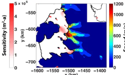
Figure 3. Adjoint sensitivity of loss of VAF to basal melting under the ice shelves adjacent to Smith Glacier (location shown in inset). Filled contours give modeled ice velocity where ice is grounded; red–white shading gives adjoint melt rate sensitivity under ice shelves. The thick black contour denotes the boundary of the ice shelves.
VAF=X
i
HAF(i)1x1y, (19)
HAF(i)=
h(i)+ρw ρ R(i)
+
, (20)
wherei is cell index,his thickness, ρ andρw are,
respec-tively, ice and ocean density,Ris bedrock elevation, and the +superscript indicates the positive part of the number. We useρ=918 kg m−3andρw=1028 kg m−3. A key aspect is
that any floating ice does not contribute to VAF.
The results are shown for the ice shelves connecting to Smith Glacier in Fig. 3, overlain on grounded ice veloc-ities (adjoint melt rate sensitivveloc-ities are zero where ice is grounded). It is interesting to note where the sensitivities are largest, along the margins of the ice shelves and also along the boundary between the two main sections of the ice shelf. The mechanism is similar to that of our test experiment: the margins are where shear stress is exerted, and thinning here will lessen the backforce on grounded ice. The boundary be-tween the two sections of the ice shelf likely plays a similar role in the ice shelf force balance, as velocity shear is large in this area (not shown).
Regarding accuracy, the finite-difference approximation to the gradient cannot be found for every ice shelf cell. How-ever, we compared the adjoint sensitivity to the finite differ-ence approximation at four arbitrary locations, and relative discrepancy was on the order of 10−5. In terms of perfor-mance, this is a much larger setting than even the highest resolution examined in the test problem. The 500 m cell size leads to approximately 200 000 ice-covered cells in the do-main (which means the matrices involved, which incorporate both x andy velocities, have 400 000 rows and columns). The forward sweep has a run time of 1150 s and the reverse sweep 1778 s. Without using the LU optimization, the reverse
sweep is 2765 s. (Multiple runs on the same cluster give sim-ilar timing results.) The timing results are encouraging, indi-cating that the relative forward/adjoint timing observed in the test problem carries over to large-scale, realistic problems.
7 Discussion and conclusions
The fixed-point algorithm of Christianson (1994) has been successfully applied to the adjoint calculation of a land ice model. The algorithm is very relevant to the model code, as the bulk of the model’s computational cost is the solution of a nonlinear elliptic equation through fixed-point iteration. As many land ice models solve a similar fixed-point problem – particularly those intended to simulate fast-flowing outlet glaciers in Antarctica and Greenland – the methodology in-troduced here has potential for the application of algorithmic differentiation techniques to other ice models. The imple-mentation of the algorithm replaces a small portion of AD-generated code by handwritten code. However, this is done such that it does not interfere with the modularity offered by AD approach, and it does not require revision as model physics change.
The algorithm offers two advantages over the more straightforward mechanical adjoint, i.e., the application of AD without intervention. First, the code solves the true ad-joint to the fixed-point iteration, rather than an approxima-tion (cf. Eq. 9). This avoids inaccurate results arising from bad initial guesses, and ensures proper convergence of the fixed-point adjoint. Second, the memory requirements do not increase with the number of adjoint iterations as they do with the mechanical adjoint. In the case of OpenAD, the effect on timing performance is small; but for machines with limited memory or for larger problems, the large memory load asso-ciated with the mechanical adjoint will be a serious issue.
As mentioned in the introduction, it is possible to differ-entiate the stress balance of an ice model at the differential equation level rather than the code level. Such approaches, however, (a) cannot make use of forward equation solvers, (b) remove somewhat the modularity of the AD approach, and (c) are not suitable for hybrid models, which are being popular due to their balance between generality and com-putational expense. Thus we argue that our application of the Christianson fixed-point algorithm in our algorithmically dif-ferentiated ice model framework represents a contribution to land ice modeling in general.
Copyright statement
The submitted work has been created by UChicago Argonne, LLC, Operator of Argonne National Laboratory (known as “Argonne”). Argonne, a US Department of Energy Office of Science laboratory, is operated under Contract No. DE-AC02-06CH11357. The US Government retains for itself, and others acting on its behalf, a paid-up, nonexclusive, ir-revocable worldwide license in said article to reproduce, pre-pare derivative works, distribute copies to the public, and per-form publicly and display publicly, by or on behalf of the Government.
Code availability
All code necessary to carry out the experiments is publicly available through the MITgcm, OpenAD, and PETSc web-sites. Please see the Supplement to the paper for detailed in-structions regarding installation and running of experiments.
The Supplement related to this article is available online at doi:10.5194/gmd-9-1891-2016-supplement.
Acknowledgements. This work was made possible in part through a SAGES (Scottish Alliance for Geoscience, Environment and Society) travel grant for early career exchange, NERC grant NE/M003590/1, ARCHER Embedded CSE support grant eCSE03-09, and by a grant from the US Department of Energy, Office of Science, under contract DE-AC02-06CH11357. We are grateful for valuable input from Editor Ham, Referee Christianson, and one anonymous referee. Additionally the authors are grateful for valuable input from B. Smith, J. Brown, and P. Heimbach.
Edited by: D. Ham
References
Arthern, R. J., Hindmarsh, R. C. A., and Williams, C. R.: Flow speed within the Antarctic ice sheet and its controls inferred from satellite observations, J. Geophys. Res.-Earth, 120, 1171–1188, doi:10.1002/2014JF003239, 2015.
Bartholomew-Biggs, M., Brown, S., Christianson, B., and Dixon, L.: Automatic differentiation of algorithms, J. Comput. Appl. Math., 124, 171–190, doi:10.1016/S0377-0427(00)00422-2, 2000.
Blatter, H.: Velocity and stress fields in grounded glaciers: a simple algorithm for including deviatoric stress gradients, J. Glaciol., 41, 333–344, 1995.
Christianson, B.: Reverse accumulation and attractive fixed points, Optim. Method. Softw., 3, 311–326, doi:10.1080/10556789408805572, 1994.
Christianson, B.: Reverse accumulation and implicit functions, Optim. Method. Softw., 9, 307–322, doi:10.1080/10556789808805697, 1998.
Cornford, S. L., Martin, D. F., Graves, D. T., Ranken, D. F., Le Brocq, A. M., Gladstone, R. M., Payne, A. J., Ng, E. G., and Lipscomb, W. H.: Adaptive Mesh, Finite Volume Mod-eling of Marine Ice Sheets, J. Comput. Phys., 232, 529–549, doi:10.1016/j.jcp.2012.08.037, 2013.
Cuffey, K. and Paterson, W. S. B.: The Physics of Glaciers, Butter-worth Heinemann, Oxford, 4th Edn., 2010.
Dupont, T. K. and Alley, R.: Assessment of the importance of ice-shelf buttressing to ice-sheet flow, Geophys. Res. Lett., 32, L04503, doi:10.1029/2004GL022024, 2005.
Errico, R. M.: What is an adjoint model?, B. Am. Meteorol. Soc., 78, 2577–2591, 1997.
Favier, L., Durand, G., Cornford, S. L., Gudmundsson, G. H., Gagliardini, O., Gillet-Chaulet, F., Zwinger, T., Payne, A., and Brocq, A. M. L.: Retreat of Pine Island Glacier controlled by marine ice-sheet instability, Nature Climate Change, 4, 117–121, doi:10.1038/nclimate2094, 2014.
Forth, S., Hovland, P., Phipps, E., Utke, J., and Walther, A. (Eds.): Recent Advances in Algorithmic Differentiation, Vol. 87 of Lec-ture Notes in Computational Science and Engineering, Springer, Berlin Heidelberg, doi:10.1007/978-3-642-30023-3, 2012. Fretwell, P., Pritchard, H. D., Vaughan, D. G., Bamber, J. L.,
Bar-rand, N. E., Bell, R., Bianchi, C., Bingham, R. G., Blankenship, D. D., Casassa, G., Catania, G., Callens, D., Conway, H., Cook, A. J., Corr, H. F. J., Damaske, D., Damm, V., Ferraccioli, F., Fors-berg, R., Fujita, S., Gim, Y., Gogineni, P., Griggs, J. A., Hind-marsh, R. C. A., Holmlund, P., Holt, J. W., Jacobel, R. W., Jenk-ins, A., Jokat, W., Jordan, T., King, E. C., Kohler, J., Krabill, W., Riger-Kusk, M., Langley, K. A., Leitchenkov, G., Leuschen, C., Luyendyk, B. P., Matsuoka, K., Mouginot, J., Nitsche, F. O., Nogi, Y., Nost, O. A., Popov, S. V., Rignot, E., Rippin, D. M., Rivera, A., Roberts, J., Ross, N., Siegert, M. J., Smith, A. M., Steinhage, D., Studinger, M., Sun, B., Tinto, B. K., Welch, B. C., Wilson, D., Young, D. A., Xiangbin, C., and Zirizzotti, A.: Bedmap2: improved ice bed, surface and thickness datasets for Antarctica, The Cryosphere, 7, 375–393, doi:10.5194/tc-7-375-2013, 2013.
Giering, R., Kaminski, T., and Slawig, T.: Generating efficient derivative code with TAF adjoint and tangent linear Euler flow around an airfoil, Future Gener. Comp. Sy., 21, 1345–1355, doi:10.1016/j.future.2004.11.003, 2005.
Goldberg, D. N.: A variationally-derived, depth-integrated approxi-mation to a higher-order glaciologial flow model, J. Glaciol., 57, 157–170, 2011.
Goldberg, D. N. and Heimbach, P.: Parameter and state estima-tion with a time-dependent adjoint marine ice sheet model, The Cryosphere, 7, 1659–1678, doi:10.5194/tc-7-1659-2013, 2013. Goldberg, D. N. and Sergienko, O. V.: Data assimilation
us-ing a hybrid ice flow model, The Cryosphere, 5, 315–327, doi:10.5194/tc-5-315-2011, 2011.
Greve, R. and Blatter, H.: Dynamics of Ice Sheets and Glaciers, Springer, Dordrecht, 2009.
Griewank, A. and Walther, A.: Algorithm 799: Revolve: An Im-plementation of Checkpointing for the Reverse or Adjoint Mode of Computational Differentiation, ACM Trans. Math. Softw., 26, 19–45, doi:10.1145/347837.347846, 2000.
Griewank, A. and Walther, A.: Evaluating Derivatives. Principles and Techniques of Algorithmic Differentiation, Vol. 19 of Fron-tiers in Applied Mathematics, SIAM, Philadelphia, 2nd Edn., 2008.
Heimbach, P.: The MITgcm/ECCO adjoint modeling infrastructure, CLIVAR Exchanges, 13, 13–17, 2008.
Heimbach, P. and Bugnion, V.: Greenland ice-sheet volume sen-sitivity to basal, surface and initial conditions derived from an adjoint model, Ann. Glaciol., 50, 67–80, 2009.
Heimbach, P., Hill, C., and Giering, R.: Automatic Generation of Efficient Adjoint Code for a Parallel Navier-Stokes Solver, in: Computational Science ICCS 2002, Vol. 2331, part 3 of Lecture Notes in Computer Science, edited by: Dongarra, J. J., Sloot, P. M. A., and Tan, C. J. K., 1019–1028, Springer-Verlag, 2002. Hutter, K.: Theoretical Glaciology, Dordrecht, Kluwer Academic
Publishers, 1983.
Isaac, T., Petra, N., Stadler, G., and Ghattas, O.: Scalable and ef-ficient algorithms for the propagation of uncertainty from data through inference to prediction for large-scale problems, with ap-plication to flow of the Antarctic ice sheet, J. Comput. Phys., 296, 348–368, doi:10.1016/j.jcp.2015.04.047, 2015.
Joughin, I., Tulaczyk, S., Bamber, J. L., Blankenship, D., Holt, J. W., Scambos, T., and Vaughan, D. G.: Basal conditions for Pine Island and Thwaites Glaciers, West Antarctica, determined using satellite and airborne data, J. Glaciol., 55, 245–257, 2009. Khazendar, A., Rignot, E., and Larour, E.: Larsen B ice shelf rhe-ology preceding its disintegration inferred by a control method, Geophys. Res. Lett., 34, L19503, doi:10.1029/2007GL030980, 2007.
Larour, E., Rignot, E., Joughin, I., and Aubry, D.: Rheology of the Ronne Ice Shelf, Antarctica, inferred from satellite radar inter-ferometry data using an inverse control method, Geophys. Res. Lett., 32, L05503, doi:10.1029/2004GL021693, 2005.
Larour, E., Utke, J., Csatho, B., Schenk, A., Seroussi, H., Morlighem, M., Rignot, E., Schlegel, N., and Khazendar, A.: Inferred basal friction and surface mass balance of the North-east Greenland Ice Stream using data assimilation of ICESat (Ice Cloud and land Elevation Satellite) surface altimetry and ISSM (Ice Sheet System Model), The Cryosphere, 8, 2335–2351, doi:10.5194/tc-8-2335-2014, 2014.
Lipscomb, W., Bindschadler, R., Bueler, E., Holland, D. M., John-son, J., and Price, S.: A Community Ice Sheet Model for Sea Level Prediction, EOS T. Am. Geophys. Un., 90, p. 23, doi:10.1029/2009EO030004, 2009.
Little, C. M., Oppenheimer, M., Alley, R. B., Balaji, V., Clarke, G. K. C., Delworth, T. L., Hallberg, R., Holland, D. M., Hulbe, C. L., Jacobs, S. S., Johnson, J. V., Levy, H., Lipscomb, W. H., Marshall, S. J., Parizek, B. R., Payne, A. J., Schmidt, G. A., Stouffer, R. J., Vaughan, D. G., and Winton, M.: Toward a New Generation of Ice Sheet Models, EOS T. Am. Geophys. Un., 88, 578–579, 2007.
MacAyeal, D. R.: Large-scale ice flow over a viscous basal sed-iment: Theory and application to Ice Stream B, Antarctica, J. Geophys. Res.-Sol. Ea., 94, 4071–4087, 1989.
MacAyeal, D. R.: The basal stress distribution of Ice Stream E, Antarctica, inferred by control methods, J. Geophys. Res., 97, 595–603, 1992.
MacAyeal, D. R., Bindschadler, R. A., and Scambos, T. A.: Basal friction of Ice Stream E, West Antarctica, J. Glaciol., 41, 247– 262, 1995.
Martin, N. and Monnier, J.: Adjoint accuracy for the full Stokes ice flow model: limits to the transmission of basal friction variability to the surface, The Cryosphere, 8, 721–741, doi:10.5194/tc-8-721-2014, 2014.
McGovern, J., Rutt, I., Utke, J., and Murray, T.: ADISM v.1.0: an adjoint of a thermomechanical ice-sheet model obtained using an algorithmic differentiation tool, Geosci. Model Dev. Discuss., 6, 5251–5288, doi:10.5194/gmdd-6-5251-2013, 2013.
McMillan, M., Shepherd, A., Sundal, A., Briggs, K., Muir, A., Ridout, A., Hogg, A., and Wingham, D.: Increased ice losses from Antarctica detected by CryoSat-2, Geophys. Res. Lett., 41, 3899–3905, doi:10.1002/2014GL060111, 2014.
Morland, L. W.: Unconfined ice-shelf flow, in: Dynamics of the West Antarctic Ice Sheet, edited by: der Veen, C. J. V. and Oer-lemans, J., 99–116, Reidel Publ. Co., 1987.
Morlighem, M., Rignot, E., Seroussi, G., Larour, E., Ben Dhia, H., and Aubry, D.: Spatial patterns of basal drag inferred using con-trol methods from a full-Stokes and simpler models for Pine Is-land Glacier, West Antarctica, Geophys. Res. Lett., 37, L14502, doi:10.1029/2010GL043853, 2010.
Naumann, U.: The Art of Differentiating Computer Programs: An Introduction to Algorithmic Differentiation, no. 24 in Software, Environments, and Tools, SIAM, Philadelphia, PA, 2012. Pattyn, F.: A new three-dimensional higher-order
thermomechan-ical ice-sheet model: basic sensitivity, ice-stream development and ice flow across subglacial lakes, J. Geophys. Res.-Sol. Ea., 108, 2382, doi:10.1029/2002JB002329, 2003.
Pattyn, F., Perichon, L., Aschwanden, A., Breuer, B., de Smedt, B., Gagliardini, O., Gudmundsson, G. H., Hindmarsh, R. C. A., Hubbard, A., Johnson, J. V., Kleiner, T., Konovalov, Y., Martin, C., Payne, A. J., Pollard, D., Price, S., Rückamp, M., Saito, F., Soucek, O., Sugiyama, S., and Zwinger, T.: Benchmark experi-ments for higher-order and full-Stokes ice sheet models (ISMIP– HOM), The Cryosphere, 2, 95–108, doi:10.5194/tc-2-95-2008, 2008.
Perego, M., Price, S., and Stadler, G.: Optimal initial conditions for coupling ice sheet models to Earth system models, J. Geophys. Res.-Earth, 119, 1894–1917, doi:10.1002/2014JF003181, 2014. Petra, N., Zhu, H., Stadler, G., Hughes, T. J., and Ghattas, O.: An
Rignot, E., Mouginot, J., and Scheuchl, B.: Ice Flow of the Antarctic Ice Sheet, Science, 333, 1427–1430, doi:10.1126/science.1208336, 2011.
Rommelaere, V.: Large-scale rheology of the Ross Ice Shelf, Antarctica, computed by a control method, J. Glaciol., 24, 694– 712, 1997.
Schoof, C. and Hindmarsh, R. C. A.: Thin-Film Flows with Wall Slip: An Asymptotic Analysis of Higher Order Glacier Flow Models, Q. J. Mech. Appl. Math., 63, 73–114, 2010.
Sergienko, O. V., Bindschadler, R. A., Vornberger, P. L., and MacAyeal, D. R.: Ice stream basal conditions from block-wise surface data inversion and simple regression models of ice stream flow: Application to Bindschadler Ice Stream, J. Geophys. Res., 113, F04010, doi:10.1029/2008JF001004, 2008.
Shepherd, A., Wingham, D. J., and Mansley, J.: Inland thinning of the Amundsen Sea sector, West Antarctica, Geophys. Res. Lett., 29, L1364, doi:10.1029/2001GL014183, 2002.
Shepherd, A., Wingham, D. J., and Rignot, E.: Warm ocean is erod-ing West Antarctic Ice Sheet, Geophys. Res. Lett., 31, L23402, doi:10.1029/2004GL021106, 2004.
Taftaf, A., Hascoët, L., and Pascual, V.: Implementation and mea-surements of an efficient Fixed Point Adjoint, in: EUROGEN 2015, ECCOMAS, GLASGOW, UK, 2015.
Utke, J., Naumann, U., Fagan, M., Tallent, N., Strout, M., Heim-bach, P., Hill, C., Ozyurt, D., and Wunsch, C.: OpenAD/F: A modular open source tool for automatic differentiation of For-tran codes, ACM Transactions on Mathematical Software, 34, 18, doi:10.1145/1377596.1377598, 2008.
Vaughan, D. G. and Arthern, R.: Why Is It Hard to Pre-dict the Future of Ice Sheets?, Science, 315, 1503–1504, doi:10.1126/science.1141111, 2007.