https://doi.org/10.5194/gmd-10-3145-2017 © Author(s) 2017. This work is distributed under the Creative Commons Attribution 3.0 License.
MicroHH 1.0: a computational fluid dynamics code for direct
numerical simulation and large-eddy simulation of atmospheric
boundary layer flows
Chiel C. van Heerwaarden1,2, Bart J. H. van Stratum1,2, Thijs Heus3, Jeremy A. Gibbs4, Evgeni Fedorovich5, and Juan Pedro Mellado2
1Meteorology and Air Quality Group, Wageningen University, Wageningen, the Netherlands 2Max Planck Institute for Meteorology, Hamburg, Germany
3Cleveland State University, Cleveland, OH, USA
4Department of Mechanical Engineering, University of Utah, Salt Lake City, UT, USA 5University of Oklahoma, Norman, OK, USA
Correspondence to:Chiel C. van Heerwaarden ([email protected]) Received: 17 February 2017 – Discussion started: 21 March 2017
Revised: 19 June 2017 – Accepted: 26 June 2017 – Published: 28 August 2017
Abstract. This paper describes MicroHH 1.0, a new and open-source (www.microhh.org) computational fluid dynam-ics code for the simulation of turbulent flows in the atmo-sphere. It is primarily made for direct numerical simulation but also supports large-eddy simulation (LES). The paper covers the description of the governing equations, their nu-merical implementation, and the parameterizations included in the code. Furthermore, the paper presents the validation of the dynamical core in the form of convergence and con-servation tests, and comparison of simulations of channel flows and slope flows against well-established test cases. The full numerical model, including the associated parameteriza-tions for LES, has been tested for a set of cases under stable and unstable conditions, under the Boussinesq and anelas-tic approximations, and with dry and moist convection under stationary and time-varying boundary conditions. The paper presents performance tests showing good scaling from 256 to 32 768 processes. The graphical processing unit (GPU)-enabled version of the code can reach a speedup of more than an order of magnitude for simulations that fit in the memory of a single GPU.
1 Introduction
In this paper, we present a description of MicroHH 1.0, a new computational fluid dynamics code for the simulation of turbulent flows in doubly periodic domains, with a focus on those in the atmosphere. MicroHH is designed for the direct numerical simulation (DNS) technique but also sup-ports the large-eddy simulation (LES) technique. Its appli-cations range from neutral channel flows to cloudy atmo-spheric boundary layers in large domains. MicroHH is writ-ten in C++and the graphical processing unit (GPU)-enabled
parts of the code in NVIDIA’s CUDA. The simulation algo-rithms have been designed and are written from scratch with the goal to create a fast and highly parallel code that is able to run on machines with more than 10 000 cores. It is a key requirement for the code to be able to perform DNS at very high Reynolds numbers or to conduct LES at very fine grids (grid spacing less than 1 m), or in domains that approach the synoptic scales (beyond 1000 km). We decided to start from scratch, in order to be able to use C++and its extensive
pos-sibilities in object-oriented and metaprogramming. Further-more, the implementation of a dynamical core that is fully fourth order in space, which is very beneficial for DNS, but to retain the option to switch to second-order accuracy for LES, required a new code design.
(Heus et al., 2010), UCLA-LES (Stevens et al., 2005), and PALM (Maronga et al., 2015), deserve a reference as Mi-croHH could not have been possible without those.
This paper is built up as follows: in Sect. 2, we provide a full description of the governing equations of the dynam-ical core, and their numerdynam-ical implementation is discussed in Sect. 3. Subsequently, in Sect. 4, we present the parame-terizations and their underlying assumptions. Section 5 dis-cusses the technical details of the code, and Sects. 6 and 7 explain how to run the model and which output is gener-ated. This is followed by a series of model tests on the va-lidity and accuracy of the dynamical core in Sect. 8, and a series of more applied atmospheric flow cases based on pre-vious studies (Sect. 9). Hereafter, the parallel performance is evaluated (Sect. 10). Then, an overview of published work with MicroHH is presented (Sect. 11), followed by the future plans (Sect. 12) and the concluding remarks (Sect. 13). Fi-nally, there is a short description of where to get MicroHH, and where to find its tutorials and a selection of visualizations (see code availability section).
2 Dynamical core: governing equations
The dynamical core of MicroHH solves the conservation equations of mass, momentum, and energy under the anelas-tic approximation (Bannon, 1996). Under this approxima-tion, the state variables density, pressure, and temperature are described as small fluctuations (denoted with a prime in this paper) from corresponding vertical reference profiles (denoted with subscript zero) that are functions of height only. This form of the approximation directly simplifies to the Boussinesq approximation if the reference densityρ0(z) is taken to be constant with heightz. Consequently, MicroHH does not need separate implementations of Boussinesq and anelastic approximations. To facilitate the subsequent discus-sion of the conservation equations, we define the scale height for densityHρ based on the reference density profile:
Hρ≡
1
ρ0 dρ0
dz
−1
. (1)
2.1 Conservation of mass
The conservation of mass is formulated using Einstein sum-mation as
∂ρ0ui ∂xi
=ρ0∂ui ∂xi
+ρ0wHρ−1=0, (2)
where ui represents the components of the velocity vector (u, v, w) andxi represents the components of the position vector (x, y, z). This formulation conserves the reference mass, as density perturbations are ignored in the equation (Lilly, 1996).
Under the Boussinesq approximation (Hρ → ∞), Eq. (2)
simplifies to conservation of volume: ∂ui
∂xi =0. (3)
2.2 Thermodynamic relations and conservation of momentum
The thermodynamic relation between the fluctuations of vir-tual potential temperature, pressure, and density under the anelastic approximation is (see Bannon, 1996 for its deriva-tion)
θv0 θv0 =
p0 ρ0gHρ
−ρ
0
ρ0, (4)
whereθv0 is the perturbation virtual potential temperature,θv0 the reference virtual potential temperature,p0 is the pertur-bation pressure,g is the gravity acceleration, andρ0 is the perturbation density.
The corresponding momentum equation is written in the flux form in order to assure momentum conservation. The hy-drostatic balance dp0/dz= −ρ0g has been subtracted, and Eq. (4) has been used to introduce potential temperature as the buoyancy variable to formulate the conservation of mo-mentum as
∂ui ∂t = −
1 ρ0
∂ρ0uiuj ∂xj −
∂ ∂xi
p0 ρ0
+δi3gθ 0 v θv0+ν
∂2ui ∂xj2
+Fi, (5)
whereδ is the Kronecker delta,ν is the kinematic viscos-ity, and vectorFi represents external forces resulting from parameterizations or large-scale forcings. As Bannon (1996) showed, this formulation is energy-conserving in the sense that there is a consistent transfer between kinetic and poten-tial energy.
Under the Boussinesq approximation, the two equations simplify to
θv0 θv0 = −
ρ0
ρ0, (6)
∂ui ∂t = −
∂uiuj ∂xj
− 1
ρ0 ∂p0 ∂xi
+δi3g θv0 θv0+ν
∂2ui ∂xj2
+Fi. (7)
2.3 Pressure equation
and take its divergence. Conservation of mass ensures that the tendency term vanishes, and an elliptic equation for pres-sure remains:
∂ ∂xi
ρ0 ∂ ∂xi
p0
ρ0
=∂ρ0f (ui)
∂xi
. (8)
Under the Boussinesq approximation, the equation simplifies to
∂2 ∂xi2
p0
ρ0
=∂f (ui)
∂xi
. (9)
In Sect. 3, we explain how these equations are solved numer-ically.
2.4 Conservation of an arbitrary scalar
The conservation equation of an arbitrary scalarφis written in flux form:
∂φ ∂t = −
1 ρ0
∂ρ0ujφ ∂xj
+κφ ∂2φ ∂xj2
+Sφ, (10)
where κφ is the diffusivity of the scalar and Sφ represents sources and sinks of the variable.
2.5 Conservation of energy
MicroHH provides multiple options for the energy conserva-tion equaconserva-tion. The conservaconserva-tion equaconserva-tion for potential tem-perature for dry dynamicsθcan be written as
∂θ ∂t = −
1 ρ0
∂ρ0ujθ ∂xj
+κθ ∂2θ ∂xj2
+ θ0
ρ0cpT0
Q, (11)
where κθ is the thermal diffusivity for heat, and Q repre-sents external sources and sinks of heat. A second option for moist dynamics is available. This has an identical conserva-tion equaconserva-tion, but with liquid water potential temperatureθl rather thanθas the conserved variable (see Sect. 3.9 for de-tails).
A third, more simplified mode, is available for dry dynam-ics under the Boussinesq approximation. Here, the equation of state (Eq. 6) can be eliminated and the conservation of momentum and energy can be written in terms of buoyancy b≡(g/θv0) θv0as
∂ui ∂t +
∂uiuj ∂xj
= −1
ρ0 ∂p0 ∂xi
+δi3b+ν∂ 2u
i
∂xj2, (12) ∂b
∂t + ∂buj
∂xj
=κb ∂2b ∂x2j
+Qb, (13)
withκb as the diffusivity for buoyancy andQb as an exter-nal buoyancy source. By using buoyancy, length and time remain as the only two dimensions, which proves convenient
for dimensional analysis. In this formulation,θv0is the fluctu-ation of the virtual potential temperature with respect to the surface valueθv0. The consequence is that the buoyancy in-creases with height in a stratified atmosphere, analogously to the virtual potential temperature (see Garcia and Mellado, 2014, their Fig. B1 and van Heerwaarden and Mellado, 2016, their Fig. 7a)
With a slight modification to the definition ofθv0, it is pos-sible to study slope flows in periodic domains. We defineθv0 as the fluctuation with respect to a linearly stratified back-ground profileθv0+(dθv/dz)0z. The background
stratifica-tion in units of buoyancy isN2≡(g/θv0) (dθv/dz)0. If we work out the governing equations again and introduce a slope α (x axis pointing upslope; see Fedorovich and Shapiro, 2009, their Fig. 1) in thexdirection, we find
∂u ∂t +
∂uju ∂xj
= −1
ρ0 ∂p0
∂x +sin(α)b+ν ∂2u
∂xj2, (14) ∂w
∂t + ∂ujw
∂xj
= −1
ρ0 ∂p0
∂z +cos(α)b+ν ∂2w
∂xj2, (15) ∂b
∂t + ∂buj
∂xj
=κb ∂2b ∂xj2
−(usin(α)
+wcos(α)) N2+Qb, (16)
where the evolution equation ofvis omitted, as it contains no changes.
3 Dynamical core: numerical implementation 3.1 Grid
MicroHH is discretized on a staggered Arakawa C-grid, where the scalars are located in the center of a grid cell and the three velocity components are at the faces. The code can work with stretched grids in the vertical dimension. The grid is initialized from a vertical profile that contains the heights of the cell centers. The locations of the faces are determined consistently with the spatial order of the interpolations that are described in Sect. 3.4. All spatial operators in the model, such as the advection and diffusion, default to the same or-der as the grid and can be overridden according to the user’s wishes (see Sect. 6).
There is the option to apply a uniform translation velocity to the grid and thus to let the grid move with the flow. This so-called Galilean transformation is allowed as the Navier– Stokes equations are invariant under translation. It has the potential to allow for larger time steps and to increase the accuracy of simulations.
3.2 Three-dimensional fields
or 7) and the thermodynamic variables (Eqs. 11, 13, or 16). Furthermore, the user has the option to define additional pas-sive scalars (Eq. 10). Each of the prognostic fields has an ad-ditional three-dimensional field assigned to store its tendency (see Sect. 3.3). Furthermore, a diagnostic field is assigned for the pressure, as well as three or four additional ones for in-termediate computations. Newly implemented physical pa-rameterizations have the option to request additional three-dimensional fields at initialization of the specific parameter-ization.
The generation of turbulence requires perturbations to the initial fields. MicroHH has two options to superimpose per-turbations on any of the prognostic variables. These pertur-bations can be random noise of which the amplitude and lo-cation can be controlled, as well as two-dimensional rotating vortices with an axis aligned with thexorydimension. The former option is the most commonly used method to start convective turbulence, whereas the latter is the default for neutral or stably stratified flows, which develop turbulence more easily from larger perturbations.
3.3 Time integration
The prognostic equations are solved using low-storage Runge–Kutta time integration schemes. Such schemes re-quire two fields per variable: one that contains the ac-tual value, which we denote with φ in this section, and one that represents the tendencies, denoted with δφ. The code provides two options: a three-stage, third-order scheme (Williamson, 1980) and a five-stage, fourth-order scheme (Carpenter and Kennedy, 1994). Both can be written in the same generic form in semi-discrete formulation as
(δφ)n=f (φn)+an(δφ)n−1 (17) φn+1=φn+bn1t (δφ)n, (18) wheref is a function that represents the computation of all right-hand-side terms,anandbn are the coefficients for the Runge–Kutta method at stage n, and 1t is the time step. Expression f (φn)thus represents the actual tendency cal-culated using, for instance, Eqs. (5) or (10), whereas(δφ)nis a composite of the actual tendency and those from the ous stages. In low-storage form, the tendencies of the previ-ous stage(δφ)n−1are retained and multiplied withanat the beginning of a stage, except for the first stage, wherea1=0.
For the third-order scheme, the vectorsanandbnare
an=
0,−5
9,− 153 128
, (19)
bn=
1
3, 15 16,
8 15
. (20)
For the fourth-order scheme, the vectorsaandbare
an=
0,−567301805773
1357537059087,−
2404267990393 2016746695238,
−3550918686646
2091501179385,−
1275806237668 842570457699
(21)
bn=
1432997174477
9575080441755,
5161836677717 13612068292357,
1720146321549 2090206949498, 3134564353537
4481467310338,
2277821191437 14882151754819
. (22)
The reduced truncation error of the fourth-order scheme makes the scheme preferable over the third-order scheme un-der many conditions (see Sect. 8.2). The code can be run with a fixed1t, as well as an adaptive time step based on the local flow velocities.
3.4 Building blocks of the spatial discretization
The spatial operators are based on finite differences. The code supports second-order and fourth-order accurate dis-cretizations following Morinishi et al. (1998) and Vasilyev (2000). From Taylor series, spatial operators can be derived that constitute the building blocks of more advanced oper-ators, such as the advection and diffusion operators. In the following subsections, we describe the elementary operators and the composite operators that can be derived from them. We have selected a set of examples that cover the relevant operators.
We define two second-order interpolation operators, one with a small stencil and one with a wide stencil, as
φi,j,k≈φ2xi,j,k≡ φi−1
2,j,k+φi+12,j,k
2 , (23)
φi,j,k≈φ2xLi,j,k≡ φi−3
2,j,k+φi+32,j,k
2 . (24)
Interpolations are marked with a bar. The superscript indi-cates the spatial order (2) and the direction (x), and has an extra qualifierLwhen it is taken using the wide stencil. The subscript indicates the position on the grid (i, j).
The gradient operators, denoted with letterδ, are defined in a similar way:
∂φ ∂x
i,j,k
≈δ2x(φ)i,j,k≡
φi+1
2,j,k−φi−12,j,k
xi+1 2 −xi−12
(25)
∂φ ∂x
i,j,k
≈δ2xL(φ)i,j,k≡
φi+3
2,j,k−φi−32,j,k
xi+3 2 −xi−32
. (26)
We use the Einstein summation in the operators. For in-stance, the divergence of vector ui|i,j,k can be written as δ2xi(u
The fourth-order operators, written down in the same no-tation, are defined as
φi,j,k≈φ 4x i,j,k
≡ −φi−3
2,j,k+9φi−12,j,k+9φi+12,j,k−φi+32,j,k
16 . (27)
The biased version of this operator (suffix b in the super-script) can be applied in the vicinity of the boundaries at the bottom and top. Here, we show the biased stencil that can be applied for vertical interpolation near the bottom:
φi,j,k≈φ4zbi,j,k
≡
5φi,j,k−12+15φi,j,k+12−5φi,j,k+32+φi,j,k+52
16 . (28)
Note that we only write down the bottom boundary for brevity.
The centered and biased fourth-order gradient operators are ∂φ ∂x i,j,k
≈δ4x(φ)i,j,k
≡ φi−3
2,j,k−27φi−12,j,k+27φi+12,j,k−φi+32,j,k xi−3
2−27xi−12+27xi+12−xi+32
, (29) and ∂φ ∂z i,j,k
≈δ4zb(φ)i,j,k
≡
−23φi,j,k−1
2+21φi,j,k+12+3φi,j,k+32−φi,j,k+52
−23zk−1
2+21zk+12+3zk+32−zk+52
. (30) 3.5 Boundary conditions
The lateral boundaries in MicroHH are periodic. The bottom and top boundary conditions can be formulated in their most general form as the Robin boundary condition:
aφs+b ∂φ ∂z s
=c, (31)
witha,b, andcas constants. This gives the Dirichlet bound-ary condition whena=1,b=0, and the Neumann boundary
condition whena=0,b=1.
MicroHH makes use of ghost cells in order to avoid the need of biased schemes for single interpolation or gradi-ent operators near the wall. The values at the ghost cells are derived making use of the boundary conditions follow-ing Morinishi et al. (1998). The ghost cells for the Dirichlet boundary conditions in the second-order accurate discretiza-tion are
φ−1
2 =2c−φ12, (32)
whereas those for the Neumann boundary condition are φ−1
2 = −c
−z−1 2 +z12
+φ1
2. (33)
In the case of the fourth-order scheme, we have two ghost cells, and therefore a second boundary condition is required. Here, we set the third derivative equal to zero following Morinishi et al. (1998). For the Dirichlet boundary condition we then acquire the following expressions for the ghost cells:
φ−1 2 =
8c−6φ1 2 +φ32
3 , (34)
φ−3
2 =8c−6φ12 +φ32, (35)
whereas in the case of a Neumann boundary condition, we find
φ−1 2 = −c
z−3
2−27z−12+27z12 −z32
24 +φ12, (36)
φ−3 2 = −3c
z−3
2 −27z−12 +27z12 −z32
24 +φ32. (37)
3.6 Advection
We use the previously introduced notation to describe the more complex operators and expand them for illustration. The advection term is discretized in the flux form, whereφis an arbitrary scalar located in the center of the grid cell. In the second-order case, this gives the following discretization:
∂uφ ∂x i,j,k + ∂vφ ∂y i,j,k
≈δ2xuφ2x i,j,k
+δ2yvφ2y i,j,k
=
ui+1 2,j,kφ
2x
i+12,j,k−ui−12,j,kφ 2x i−12,j,k
xi+1 2−xi−12
+
vi,j+1 2,kφ
2y
i,j+12,k−vi,j−12,kφ 2y i,j−12,k
yj+1 2−yj−12
. (38) The discretization of the advection of the velocity compo-nents (see Eqs. 5 and 7) involves extra interpolations as the following example illustrates:
∂vu ∂x i,j,k
=δ2xv2yu2x i,j,k
=
v2y i+12,j,ku
2x
i+12,j,k−v 2y i−12,j,ku
2x i−12,j,k
xi+1 2−xi−12
. (39) In the standard fourth-order scheme, the scalar advection in flux form is represented by
∂uφ ∂x i,j,k
≈δ4xuφ4x i,j,k
=ui−3 2,j,kφ
4x
i−32,j,k−27ui−12,j,kφ 4x i−12,j,k
+27u
i+12,j,kφ 4x
i+12,j,k−ui+32,j,kφ 4x i+32,j,k
.
xi−3
2−27xi−12+27xi+12−xi+32
MicroHH has a fully kinetic energy-conserving fourth-order advection scheme (Morinishi et al., 1998) available. The scheme is constructed by interpolation of two kinetic energy-conserving second-order discretizations to eliminate the second-order error (as illustrated below)
∂uφ ∂x
i,j,k
≈9
8δ2x
uφ2x i,j,k
−1
8δ2xL
uφ2xL
i,j,k, (41) to ensure that velocity variances are conserved under advec-tion.
Velocity interpolations, such as those in Eq. (39), still need to be performed with fourth-order accuracy (Eq. 27) in order to be fourth-order accurate (see Morinishi et al., 1998 for details). The expression
∂vu ∂x
i,j,k
≈9
8δ2
xv4yu2x i,j,k
−1
8δ2xL
v4yu2xL
i,j,k (42)
includes, for instance, a combination of second- and fourth-order interpolations.
To increase the overall accuracy of the second-order ad-vection operator, there is an option available to only increase the interpolation part to fourth order:
∂uφ ∂x
i,j,k
≈δ2xuφ4x
i,j,k. (43)
3.7 Diffusion
We apply a discretization for diffusion that can be written as the divergence of a gradient, using the building blocks de-fined earlier in this section. As this operator is identical in all directions, we present it in one direction only:
κφ ∂2φ ∂x2
i,j,k
≈κφδ2x
δ2x(φ)
i,j,k, (44)
κφ ∂2φ ∂x2
i,j,k
≈κφδ4x
δ4x(φ)
i,j,k. (45)
On an equidistant grid, this provides the well-known second-order accurate operator for the second derivative:
κφδ2x
δ2x(φ) i,j,k
=κφ
φi−1,j,k−2φi,j,k+φi+1,j,k (1x)2 , (46) where1xis the uniform grid spacing.
For the fourth-order accurate operator, a seven-point sten-cil is used:
κφδ4x
δ4x(φ)
i,j,k
= κφ
576(1x)2 φi−3,j,k−54φi−2,j,k+783φi−1,j,k
−1460φi,j,k+783φi+1,j,k−54φi+2,j,k+φi+3,j,k
. (47) Whereas diffusion can be computed with fourth-order ac-curacy using a five-point stencil, we use a seven-point sten-cil, as it extends naturally to non-uniform grids as explained
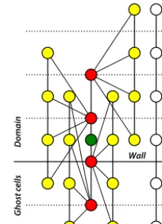
Figure 1.Schematic of the diffusion discretization near the wall.
The green node is the evaluation point at the center of the first cell above the wall, the red nodes are the stencil of the divergence ator, and yellow nodes show the stencils of the four gradient oper-ators over which the divergence is evaluated. White nodes indicate the extent of the stencil.
in Castillo et al. (1995). The usage of a seven-point stencil requires special care near the walls. In Fig. 1, we show an example of how the second derivative in the vertical direc-tion is computed for a scalar at the first model level (green node in Fig. 1). The calculation of the divergence (Fig. 1, red stencil) requires the gradient located at the first face below the wall (lowest red node in Fig. 1), which can only be ac-quired using the biased gradient operator (Eq. 30 and yellow stencil connected to lowest red node in Fig. 1). The extent of the complete stencil near the wall (white nodes; Fig. 1) is thus six points, rather than seven.
3.8 Pressure
Equations (8) and (9) are solved following the method of Chorin (1968). This is a fractional step method that first com-putes intermediate values of the velocity components for the next time step, based on all right-hand-side terms of the mo-mentum conservation equation (Eq. 5):
u∗i
t+1 i,j,k=ui|
t
i,j,k+1t fi|ti,j,k, (48) with the intermediate velocity components denoted with an asterisk.
The velocity values at the next time step can be computed as soon as the pressure is known, using
ui|ti,j,k+1 =u∗i
t+1 i,j,k−1t δ
nxi
p
ρ0
t
i,j,k
. (49)
ar-riving at δnxi(ρ
0ui)
t+1 i,j,k=δ
nxi ρ 0u∗i
t+1 i,j,k
−1t δnxi
ρ0δnxi
p
ρ0
t
i,j,k
, (50) wherenindicates the spatial order, and the subscriptiin su-perscriptxi indicates thatδnxi is a divergence operator. The left-hand side equals zero due to mass conservation at the next time step (Eq. 2). The resulting equation is the Poisson equation that is the discrete equivalent of Eq. (8). Rewriting this equation leads to
δnxi ρ0u∗ i
t+1 i,j,k 1t =δ
nxi
ρ0δnxi
p
ρ0
t
i,j,k
. (51) To simplify the notation, we denote the left-hand-side term asψand thep/ρ0term on the right-hand side asπ. Solving a Poisson equation is a global operation. Because the com-puted fields are periodic in the horizontal directions on an equidistant grid, and a Poisson equation is linear, we can per-form a Fourier transper-form in the two horizontal directions:
b
ψl,m,k= −k∗2nbπl,m,k−l
2 ∗nbπl,m,k
+δnzρ0δnz(bπ )l,m,k, (52) where Fourier-transformed variables are denoted with a hat, the spatial order of the operation withn, and the wavenum-bers in the two horizontal dimensionsx andy arel andm, respectively. Variablesk2∗andl∗2are the squares of the modi-fied wavenumbers:
−k∗22≡2
cos(k1x) (1x)2
− 2
(1x)2 (53)
and
−k∗24≡2cos(3k1x)−54cos(2k1x)+783cos(k1x)
576(1x)2
− 1460
576(1x)2, (54)
where the former is the modified wavenumber for the second-order accurate solver and the latter is the wavenumber for the fourth-order one. Note that the coefficients correspond to those in Eqs. (46) and (47). Both expressions satisfy the limit lim1x→0k2∗n=k2, wherenis the order of the scheme.
Solving Eq. (52) for bπ requires solving a banded matrix
for the vertical direction in which the walls are located. This matrix is tridiagonal for the second-order solver and hep-tadiagonal for the fourth-order solver. For this, a standard Thomas algorithm (Thomas, 1949) is used. After the pres-sure is acquired, inverse Fourier transforms are applied and subsequently the pressure gradient term (see Eqs. 5 and 7) is computed for all three components of the velocity tendency. Note that the computation of the corrected velocity compo-nents does not require a boundary condition for pressure (see Vreman, 2014 for details).
3.9 Thermodynamics
MicroHH supports the potential (θ) and liquid water poten-tial (θl) temperature as thermodynamic variables (Sect. 2.5). The dry (θ) and moist (θl) thermodynamics are related through the use of a total specific humidityqt, which is de-fined as the sum of the water vapor specific humidity (qv) and the cloud liquid water specific humidity (ql). In the absence of liquid water,θl=θ; in the presence of liquid water, the
liquid water potential temperature is approximated as (Betts, 1973)
θl≈θ− Lv
cp5
ql, (55)
whereLvis the latent heat of vaporization, cp the specific heat of dry air at constant pressure, and5is the Exner func-tion:
5=
p
p00
Rd/cp
, (56)
wherepis the hydrostatic pressure,p00a constant reference pressure, andRdthe gas constant for dry air. The cloud liquid water content is calculated as
ql=max(0, qt−qs), (57)
whereqsis the saturation specific humidity: qs= es
p−(1−) es, (58) withthe ratio between the gas constant for dry air and the gas constant for water vapor (Rd/Rv), andes the saturation vapor pressure. The latter is approximated using a 10th order Taylor expansion atT =0◦C of the Arden Buck equation
(Buck, 1981).ql is adjusted iteratively to arrive at a consis-tent state whereqv=qs. Finally, the virtual potential temper-ature (Eq. 5) is defined in MicroHH as
θv≡θ
1−
1−Rv
Rd
qt−Rv
Rdql
. (59)
The base state pressure and density are calculated assuming a hydrostatic equilibrium: dp0= −ρ0gdz, with the density de-fined asρ0=p0/(Rd5 θv0). Integration with height results in
p0;k+1=p0;kexp
−g(z
k+1−zk) Rd5 θv0
, (60)
whereθv0 is the average virtual potential temperature be-tweenzkandzk+1. This equation is applied from a given sur-face pressure to the model top, alternating the calculations at the full and half model levels. That is, given the full thermo-dynamic state (pressure and density) at a full levelk, the ther-modynamic state can be advanced from the half levelk−1
tok+12. Using the newly calculated state atk+12, pressure
and density atk+1 can be calculated.
The base state density ρ0 that is used in the dynamical core (Sect. 2) is calculated using the initial virtual potential temperature profile and is not updated during the experiment. The density and hydrostatic pressure used in the moist ther-modynamics can optionally be updated every time step, fol-lowing the same procedure as explained in Boing (2014). 3.10 Rotation
The effects of a rotating reference frame on anf plane can be included through the Coriolis force. The acceleration due to the Coriolis forceFi,coris computed for the two horizontal velocity components (indices 1 and 2 in Eqs. 5 and 7) as
F1,cori,j,k=f0vi,j,k, (61) F2,cori,j,k= −f0ui,j,k, (62) withf0as Coriolis parameter specified by the user.
4 Physical parameterizations
4.1 Subfilter-scale model for large-eddy simulation With the governing equations described in Sect. 2 it is pos-sible to resolve the flow down to the scales where molecular viscosity acts. In many applications, however, such simula-tions are too costly. In that case, one may opt for large-eddy simulation (LES), where filtered equations are used to de-scribe the largest scales of the flow, and the subfilter-scale motions are modeled. The LES implementation in MicroHH assumes very high Reynolds numbers in which the molecular viscosity is neglected. Filtering of the anelastic conservation of momentum equation (Eq. 5), with a tilde applied to denote filtered variables, leads to
∂eui ∂t = −
1 ρ0
∂ρ0euieuj
∂xj − ∂π ∂xi −
1 ρ0
∂ρ0τij ∂xj
+δi3g
eθv0
θv0+Fi. (63)
In this equation, a tensorτij is defined as τij≡ugiuj−euieuj−
1
3(ugiui−euieui) . (64)
This is the anisotropic subfilter-scale kinematic momentum flux tensor. The isotropic part of the full momentum flux ten-sor has been added to the pressure, providing the modified pressure:
π≡ ep
0
ρ0+ 1
3(uigui−euieui) . (65)
As τij contains the filtered product of unfiltered velocity components, this quantity needs to be parameterized. Mi-croHH uses the Smagorinsky–Lilly (Lilly, 1968) model, in
whichτij is modeled as
τij= −Km
∂
eui
∂xj
+∂euj
∂xi
, (66)
withKm interpreted as the subfilter eddy diffusivity. This quantity is modeled as
Km=λ2S
1−
g θv0
∂eθv
∂z
PrtS2
1 2
, (67)
and is proportional to the magnitudeS≡ 2SijSij
1 2 of the
strain tensorSij, which is defined as
Sij≡1
2
∂
eui
∂xj
+∂euj
∂xi
. (68)
The subfilter eddy diffusivity thus takes into account the lo-cal stratification and the turbulent Prandtl numberPrt. The latter is set to one-third by default but can be overridden in the settings. The length scaleλis the mixing length defined following Mason and Thomson (1992), as
1 λn =
1 [κ (z+z0)]n
+ 1
(cs1)n, (69) which is an arbitrary matching function (nis a free param-eter, set to 2 in MicroHH) between the mixing length fol-lowing wall scaling to the subfilter length scale (filter size) 1≡(1x1y1z)1/3, related to the grid spacing. The grid scale is used as an implicit filter; thus, no explicit filtering is applied. In the case of a high Reynolds number atmospheric LES with an unresolved near-wall flow, the vertical gradients of the horizontal velocity components∂eui,j/∂zin the strain tensor are replaced with the theoretical gradients predicted from Monin–Obukhov similarity theory. Evaluation of these gradients is explained in detail in Sect. 4.2.
The same approach is followed for all scalars, including the thermodynamic variables discussed in Sect. 2.5:
∂eφ
∂t = − 1 ρ0
∂ρ0eujeφ
∂xj
− 1
ρ0
∂ρ0Rφ,j ∂xj
+eSφ. (70)
The termRφ,j refers to the subfilter flux ofeφand is defined
as
Rφ,j =ujgφ−eujeφ. (71)
The subfilter-scale flux is parameterized in terms of the gra-dient
Rφ,j = − Km
Prt ∂eφ
∂xj
4.2 Surface model
The LES implementation of MicroHH uses a surface model that is constrained to rough surfaces and high Reynolds num-bers, which is a typical configuration for atmospheric flows. This model computes the surface fluxes of the horizontal momentum components and the scalars (including thermo-dynamic variables) using Monin–Obukhov similarity theory (MOST) (Wyngaard, 2010, his Sect. 10.2). MOST relates surface fluxes of variables to their near-surface gradients us-ing empirical functions that depend on the height of the first model levelz1divided by the Obukhov lengthLas an argu-ment. LengthLis defined as
L≡ − u
3 ∗
κB0, (73)
where u∗ is the friction velocity, κ is the Von Karman constant, and B0 is the surface kinematic buoyancy flux. L represents the height at which the buoyancy produc-tion/destruction of turbulence kinetic energy equals the shear production. In MicroHH, we use a local implementation of MOST, i.e., each grid point has its own value of L. This choice can lead to a overestimation of near-surface wind due to violation of the MOST assumption of horizontal homo-geneity (Bou-Zeid et al., 2005, their Fig. 18), but it allows for a more straightforward extension to heterogeneous land surfaces.
Following MOST, the friction velocityu∗and the momen-tum fluxes may be related to the near-surface wind gradient as
κz1 u∗
∂U ∂z ≈ −
κz1u∗ u0w0
∂eu ∂z ≈ −
κz1u∗ v0w0
∂ev ∂z ≈φm
z1
L
, (74) whereU is defined as
√
eu2+ev2, and u
0w0 andv0w0 as the surface momentum fluxes for the two wind components. These relationships can be integrated from the roughness lengthz0mtoz1resulting in
u∗=fm(U1−U0) , (75) u0w0= −u
∗fm(eu1−eu0) , (76)
v0w0= −u
∗fm(ev1−ev0) , (77)
withfmdefined as fm≡
κ
ln z1
z0m
−9m zL1
+9m z0Lm
, (78)
with9mdescribed in Eqs. (83) and (85).
The same procedure for scalars is followed, with κz1u∗
φ0w0 ∂φe
∂z =φh
z1
L
, (79)
and in integrated form:
φ0w0=u
∗fh eφ1−eφ0
, (80)
with fh≡
κ
lnz1
z0h
−9h zL1+9h zL0h
, (81)
with9hdescribed in Eqs. (83) and (85).
The functionsφm,φh,9m, and9h are empirical and de-pend on the static stability of the atmosphere. Under unstable conditions, we follow (Wilson, 2001; Wyngaard, 2010):
φm,h=
1+γm,h|ζ|2/3 −1/2
, (82)
9m,h=3ln
1+φm,h−1 2
!
, (83)
where ζ is the ratio of a height and the Obukhov length L,γm=3.6, andγh=7.9. Under stable conditions, we use (Högström, 1988; Wyngaard, 2010)
φm,h=1+λm,hζ, (84)
9m,h= −λm,hζ, (85)
whereλm=4.8 andλh=7.8.
With the equations above, the surface fluxes, surface val-ues, and near-surface gradients can be computed but only if the Obukhov lengthLis known. The surface model calcu-lates the Obukhov length by relating the dimensionless pa-rameterz1/L to a Richardson number. The employed for-mulation of the Richardson number depends on the chosen boundary condition in the model. Three possible options are available:
– The first option is fixed momentum fluxes and a fixed surface buoyancy flux. Both the friction velocityu∗and the surface buoyancy fluxB0are specified. Under these conditions, we define the Richardson numberRiaequal toz1/L;Lcan be computed directly from the expres-sion
Ria≡ z1 L = −
κz1B0 u3∗
. (86)
– The second option is a fixed horizontal velocityU0at the surface and a fixed surface buoyancy fluxB0. The friction velocityu∗is unknown. Now,Lneeds to be re-trieved from the implicit relationship:
Rib≡ z1 Lf
3 m= −
κz1B0
the buoyancy are given, and both u∗ and the surface buoyancy fluxB0are unknown.Lis then retrieved from
Ric≡ z1 L
fm2 fh
=κz1 eb1 −eb0
(U1−U0)2 . (88) In the event of the latter two options, a solver is required to find the value ofLthat satisfies the equation, asfm(Eq. 78) andfh (Eq. 81) both depend onLas well. For performance reasons, we have created a lookup-table-based approach that relates L to the Richardson number. The lookup table has 104 entries, of which 90 % is spaced uniformly between z1/L= −5 to 5. The remaining 10 % are used to stretch the
negative range up to z1/L= −104 to allow for the correct
free convection limit. 4.3 Large-scale forcings 4.3.1 Pressure force
MicroHH provides two options to introduce a large-scale pressure force into the model. The first is to enforce a con-stant mass flux through the domain in the streamwise direc-tion. In this approach, the desired large-scale velocityUf is set, and the corresponding pressure gradient is computed. We follow here the approach of van Reeuwijk (2007). In this ap-proach, theucomponent of the horizontal momentum equa-tion (Eq. 5) is volume averaged to acquire
huin+1− huin
1t = hf1i −
∂
∂x
p
ρ0
+Fp;ls, (89)
where brackets indicate a volume average,f1contains all the right-hand-side terms of the u component of the conserva-tion of momentum, except for the dynamic pressure, which is contained in the second term. The large-scale pressure force Fp;ls, which is to be computed, is the last term. We can now sethuin+1=Uf to explicitly set the volume-averaged veloc-ity in the next time step. Furthermore, the volume-averaged horizontal pressure gradient vanishes, because of the periodic boundary condition, which makes Fp;lsthe only unknown. The acquired pressure forceFp;lswill be added as an exter-nal force in the equation of zoexter-nal velocity (F1in Eqs. 5 and 7).
The second option is to enforce a large-scale pressure force through the geostrophic wind componentsugandvg, in com-bination with rotation, with the accelerations of the two hor-izontal velocity componentsFi,p;lscalculated as
F1,p;ls
i,j,k= −f0vg;k, (90) F2,p;ls
i,j,k=f0ug;k, (91) where ug;k and vg;k are user-specified vertical profiles of geostrophic wind components.
4.3.2 Large-scale sources and sinks
Large-scale sources and sinks, representing, for instance, large-scale advection or radiative cooling, can be prescribed for each variable separately. The user has to provide vertical profiles of large-scale sources and sinksSφ;lsthat are added to the total tendencies.
4.3.3 Large-scale vertical velocity
A second method of introducing large-scale thermodynamic effects is through the inclusion of a large-scale vertical ve-locity. In this case, each scalar gets an additional source term Sφ,w,lsof the form
Sφ,w,lsi,j,k= −wls;kδ2x hφik
, (92)
wherewls;k is a user-specified vertical profile of large-scale vertical velocity andhφik is the horizontally averaged
verti-cal profile at heightzkfor scalarφ. The tendency term is not applied to the momentum variables.
4.4 Buffer layer
MicroHH has the option to damp gravity waves in the top of the simulation domain in a so-called buffer layer. The source termSφ,bufassociated with the damping at grid celli, j, kis calculated for an arbitrary variableφas
Sφ,bufi,j,k=
φi,j,k−φ0;k τd;k
, (93)
whereφ0 is taken from a user-specified vertical reference profile, and timescaleτdis a measure for the strength of the damping. It varies with height and is calculated at heightzk following
τd−;k1=σ
z
k−zb;bot zb;top−zb;bot
β
, (94)
whereσ is the damping frequency chosen by the user andβ an exponent that describes the shape of the vertical profile of the damping frequency, which is always zero at the bottom (zb;bot) andσat the top (zb;top) of the layer.
5 Technical details of the code 5.1 Code structure
MicroHH is written in C++ and uses elements of
extensions. High performance of computational kernels is achieved by executing kernels in their own function, with explicit inclusions of therestrictkeyword to notify the compiler that fields do not overlap in memory. Furthermore, compiler-specific pragmas are used to aid vectorization on Intel compilers.
5.2 GPU
MicroHH is enabled to run on fast and energy-efficient graphical processing units (GPUs). This promising technique has been pioneered in atmospheric flows by Schalkwijk et al. (2012) and has shown its potential in weather forecasting (Schalkwijk et al., 2015). The implementation is based on NVIDIA’s CUDA. The CPU and GPU version reside in the same code base, where the GPU implementation is activated with the help of precompiler statements. The philosophy is that the entire model is initialized on the CPU and that the GPU implementation is only activated right before starting the main time loop. At that moment, the required fields are copied in double precision accuracy to the GPU, and the en-tire time integration is done there. Synchronization only hap-pens when statistics have to be computed or when restart files or cross sections of flow fields are saved to disk, to ensure high performance. The design choice to do the entire initial-ization on the CPU minimizes the amount of GPU code and therefore allows for maintaining a single code base for the CPU and GPU code.
5.3 Parallelization
The code uses the Message Passing Interface (MPI) in or-der to run on a large number of cores. The three-dimensional simulation domain is split into vertically oriented columns standing on a two-dimensional grid. The code assigns one MPI task to each grid column using the MPI_Cart_create function and uses this grid to detect the IDs of neighbor-ing processes. In order to avoid complex packneighbor-ing routines, we make use of MPI datatypes wherever possible. The MPI calls are hidden in an interface to avoid the need to manually write MPI calls.
The input/output (IO) is entirely based on MPI-IO, the parallel IO framework that comes with MPI, to ensure that three-dimensional fields and two-dimensional cross sections are stored as single files. We have chosen MPI-IO in order to limit the number of files resulting from simulations on a large number of processes and to allow for restarts on a different number of processes. In order to keep complexity of the IO as low as possible, we make use of the MPI_Sub_array function in combination with MPI_File_write_all in order to write the fields.
5.4 External dependencies
MicroHH depends on several external software tools or li-braries. It uses the CMake (https://cmake.org) build system
for the generation of Makefiles. CMake allows for paral-lel builds, which minimizes the compilation time, and it is easy to add configurations for different machines. Further-more, the FFTW3 library (Frigo and Johnson, 2005) is used for the computation of fast Fourier transforms. The statis-tical routines make use of netCDF software developed by UCAR/Unidata (http://doi.org/10.5065/D6H70CW6). In or-der to run the provided test cases and their output scripts, a Python (https://www.python.org) installation including the NumPy (van der Walt et al., 2011; http://www.numpy.org) and Matplotlib (Hunter, 2007; https://matplotlib.org) mod-ules is required. Automatic documentation generation can be done using Doxygen (http://doxygen.org), but this is op-tional.
6 Running simulations
In order to run a simulation with MicroHH, a sequence of steps needs to be taken. Each simulation has an.inifile that contains the settings of the simulation, a .prof file that contains the (initial) vertical profiles of all required variables, and, if time-varying boundary conditions are de-sired, a file with the prescribed time evolution for all time-varying boundary conditions. MicroHH provides a document (doc/input.pdf) that contains an overview of all possi-ble options that can be specified in the.inifile.
To prepare a simulation with the name test_simulation, MicroHH needs to be run in the following way:
./microhh init test_simulation
where it is assumed that test_simulation.ini and test_simulation.profare available in the directory where the command is triggered. This procedure will create the initial fields of all prognostic variables and save the re-quired fields for those model components that need to save their state to guarantee bitwise identical restarts.
After the previously described initialization phase, the ex-ecution of
./microhh run test_simulation
will start the actual simulation. Depending on the chosen out-put intervals, the simulation will create restart files, statistics, cross sections, and field dumps. MicroHH can restart from any time at which the restart files are saved.
The last mode in which the code can run is the post-processing mode. By running
./microhh post test_simulation
10−2 10−1
∆x[-] 10−12
10−10
10−8
10−6
10−4
10−2
Error
[-]
u2
u4
u4M
w2
w4
w4M
p2
p4
p4M
Figure 2.Convergence of the spatial discretization error in the
two-dimensional Taylor–Green vortex. Subscript 2 indicates the second-order scheme, subscript 4 the most accurate fourth-second-order scheme, and subscript 4Mthe fully energy-conserving fourth-order scheme. The dashed black line is the reference for second-order conver-gence; the dotted black lines indicate fourth-order convergence.
7 Model output 7.1 Statistics
A large set of output statistics can be computed during run-time at user-specified run-time intervals. The statistics mod-ule provides vertical profiles of means, second-, third- and fourth-order moments of all prognostic variables, as well as advective and diffusive fluxes. Furthermore, there are mul-tiple diagnostic variables, such as the pressure, the pres-sure variance, and its vertical flux. The thermodynamics gen-erate their own statistics based on the chosen option. The moist thermodynamics provides a large set of cloud statis-tics. There is a separate module for budget statistics, which provides the budgets of all components of the Reynolds stress tensor, and those of the variance and vertical flux of the ther-modynamic variables.
One of the key features of the MicroHH statistics routine is that an arbitrary mask can be passed into the routine over which the statistics are calculated. This allows, for instance, for a very simple way of computing conditional statistics in updrafts or clouds, which is demonstrated later in Sect. 9.2. 7.2 Two- and three-dimensional output
It is possible to save two-dimensional cross sections and three-dimensional fields of any of the prognostic and diag-nostic variables of the model, as well as of derived vari-ables. This output can be made at user-specified time inter-vals. Cross sections can be made in any chosen xy,xz, and yzplanes. Derived variables (any arbitrary function of exist-ing model variables), can be easily added to the code by the user.
100 101
∆t [-]
10−8
10−7
10−6
10−5
10−4
10−3
|
∆
KE
|
[-]
(b)
RK3
RK4 O(3)O(4)
0 200 400 600 800 1000
t [-] −0.6
−0.5 −0.4 −0.3 −0.2 −0.1 0.0
∆
KE
×
10
3[-]
(a)
RK3: dt = 10 RK4: dt = 10 RK3: dt = 5 RK4: dt = 5 RK3: dt = 2.5 RK4: dt = 2.5
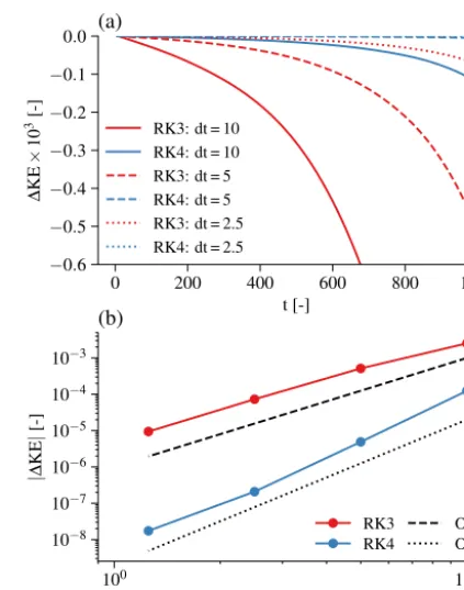
Figure 3.Time evolution of the kinetic energy change1KE during 1000 time units of random noise advection for the RK3 and RK4 time integration schemes with three different time steps(a). Kinetic
energy change convergence of the temporal discretization for the RK3 and RK4 schemes(b).
8 Validation of the dynamical core
In this section, we present a series of cases intended to vali-date MicroHH under a wide range of settings. Each of these test cases is available in the cases/directory in the Mi-croHH repository, where all detailed settings can be found (see code availability section). Below, we present only the most relevant information per case.
8.1 Taylor–Green vortex
The two-dimensional Taylor–Green vortex (cases/taylorgreen) presents an ideal test case for a dynamical core, as it has an analytical solution even though it is nonlinear. This flow is composed of two rotat-ing vortices whose evolution in a domain [0,1;0,0.5] is
described with
u(x, z, t )=sin(2π x)cos(π z)f (t ), (95)
w(x, z, t )=cos(2π x)sin(π z)f (t ), (96)
p(x, z, t )=1
4(sin(4π x)+sin(4π z)) f (t )2, (97) wheref (t )=8π2νt.
We use the analytical form att=0 as the initial
−0.12 0.00 0.12 0.24 0.36 0.48
u[m s−1]
0 3 6 9 12 15
z
[m]
(a)
Analytical MicroHH
−0.4 0.0 0.4 0.8 1.2 1.6
b[m s−2]
0 3 6 9 12 15
z
[m]
(b)
Figure 4.Normalized numerical Prandtl model solutions for
veloc-ityu(a)and buoyancyb(b)compared to their analytical
counter-parts.
ν=(800π2)−1. We compare the result against the analytical solution for a set of grid spacings and with the second-order and fourth-order dynamical cores; for the latter we compare the most accurate advection scheme and the fully energy-conserving one.
Figure 2 shows the error convergence of the sim-ulations. The error for a variable φ is computed as
P
1x1zφi,k−φref,i,k,
over the two-dimensional domain,
where1xand1zare the uniform grid spacings used in this case andφrefis the analytical solution. All variables converge according to the order of the numerical scheme. The fourth-order dynamical core loses accuracy at fine grid spacings. This is due to the boundary condition for the vertical veloc-ity that sacrifices an order of accuracy to ensure global mass conservation (Morinishi et al., 1998).
8.2 Kinetic energy conservation and time accuracy The second test of the dynamical core consists of combined evaluation of kinetic energy (KE≡12 u2+v2+w2) con-servation and time accuracy (cases/conservation). In this experiment, we run the model with only the advection and pressure solver enabled and advect random noise through the domain for 1000 s. These tests have been conducted with the third- and fourth-order Runge–Kutta schemes. We have chosen the fourth-order spatial discretization in order to demonstrate its energy conservation.
The loss of kinetic energy as a function of time is shown in Fig. 3a. The fourth-order scheme results in a smaller energy
100 101 102
0 5 10 15 20 25
h
u
i
[-]
(a)
Moser MicroHH
100 101 102
z[-] 0.0
0.5 1.0 1.5 2.0 2.5 3.0
h
u
0ui
0ii
1
/
2[-]
(b) hu0u0i hv0v0i hw0w0i
Figure 5.Velocity means(a) and variances(b) for Moser et al.
(1999) channel flow case at a Reynoldsτ of 590. The dashed ver-tical lines mark the spectra locations. Heightzis normalized with uτ/ν; velocities withu−τ1.
loss for the same time step and a faster convergence. The error-convergence plot (Fig. 3b) shows that the error con-vergence is in accordance with the order of the respective scheme. Furthermore, it illustrates the fact that, if high accu-racy in time is desired, the five-stage, fourth-order scheme is less expensive than the three-stage, third-order scheme. For instance, at a1tof 10, the error of the fourth-order scheme is approximately equal to the error of the third-order scheme at a1t of 2.5. To reach this accuracy, the fourth-order scheme needs only 5 steps per 10 time units, whereas the third-order scheme needs 12 steps.
8.3 Laminar anabatic flow
To test the buoyancy routine and the option to put the domain on a slope, a Prandtl-type anabatic slope flow (Prandtl, 1942) has been simulated (cases/prandtlslope). In this test case, the surface is inclined at an angle of 30◦and a linearly stratified atmosphere (N=1 s−1) is heated from below with
a fixed surface buoyancy flux of 0.005 m2s−3.
100 101 102
−0.4
−0.2
0.0 0.2 0.4
∂
h
u
0u 0i/
∂
t
[-]
(a)
ε S Tt
Tν
P Moser MicroHH
100 101 102
−0.15
−0.10
−0.05
0.00 0.05 0.10 0.15
∂
h
v
0v 0i/
∂
t
[-]
(b)
ε S Tt
Tν
P
100 101 102 z[-]
−0.06
−0.04
−0.02
0.00 0.02 0.04
∂
h
w
0w 0i/
∂
t
[-]
(c)
ε Tt Tν
P Tp
100 101 102 z[-]
−0.3
−0.2
−0.1
0.0 0.1 0.2 0.3
∂
h
T
K
E
i
/
∂
t
[-]
(d)
ε S
Tt Tν
Tp
Figure 6.Budgets of variances and turbulence kinetic energy (TKE, defined asu02+v02+w02/2) compared against Moser et al. (1999)’s reference data at a Reynoldsτof 590. Heightzis normalized withuτ/ν; the variances and TKE budget withν/u4τ.
8.4 Turbulent channel flow
For fully turbulent flows, the numerical solutions can-not be compared against any analytical test cases. There-fore, we validate our results against a channel flow at a Reynolds τ number of 590 (Moser et al., 1999) for means, variances, spectra, and second-order budget statis-tics (cases/moser590). The case is run at a resolution of 768×384×256 grid points. The original numerical
sim-ulation data of Moser et al. (1999) have been produced on a 384×384×256 grid with spectral schemes in the horizontal
dimensions and Chebyshev polynomials in the vertical. Figure 5a shows the normalized horizontally averaged streamwise velocity. The normalized rms values of all three velocity components are presented in Fig. 5b. All plotted variables show a perfect match with the data and are indis-tinguishable from Moser’s data. In order to further assess the accuracy of the data, we show the second-order budgets of the variances in Fig. 6. Also here, the match with the refer-ence data is excellent, which indicates that the whole range of spatial scales in the flow is represented well and that the fourth-order scheme is well able to pick up the small-scale details of the flow.
The findings in the previous paragraph are further corrobo-rated by the spectra shown in Fig. 7. Over the whole range of scales, the match between our simulation and that of Moser et al. (1999) is excellent. Note that the spectra from Moser’s simulation display an increase in pressure variance at the highest wavenumbers. This increase is the result of aliasing
errors at high wavenumbers that are typical for the spectral schemes that Moser et al. (1999) used.
8.5 Turbulent katabatic flow
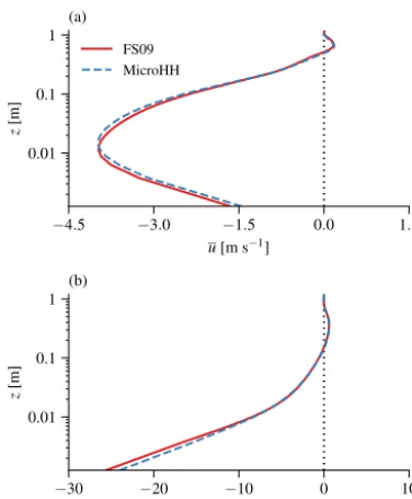
The final evaluation of the dynamical core without parame-terizations enabled is based on the direct numerical simula-tion of a turbulent katabatic flow. Here, a buoyancy-driven slope flow is simulated following the setup of Fedorovich and Shapiro (2009) (cases/drycblslope). A flow over a slope inclined at an angleαof 60◦is simulated with a fixed uniform surface buoyancy flux of −0.5 m2s−3. The
simu-lation is performed in a domain of 0.64 m×0.64 m×1.6 m
using a uniform grid of 256×256×640 points. The initial
state is a fluid at rest with a linear buoyancy stratificationN of 1 s−1. No-slip boundary conditions are applied at the bot-tom; free-slip at the top.
100 101 102 κ
10−6
10−5
10−4
10−3
10−2
10−1
100
E
[-]
(a) Streamwise,z+= 5
Euu Evv Eww Epp
Moser MicroHH
100 101 102
κ
10−6
10−5
10−4
10−3
10−2
10−1
100
(b) Spanwise,z+= 5
Euu Evv Eww Epp
100 101 102
κ
10−6
10−5
10−4
10−3
10−2
10−1
100
(c) Streamwise,z+= 99
Euu Evv Eww Epp
100 101 102
κ
10−6
10−5
10−4
10−3
10−2
10−1
100
(d) Spanwise,z+= 99
Euu Evv Eww Epp
Figure 7.Spectra of all velocity components and pressure compared against Moser et al. (1999)’s reference data at a Reynoldsτof 590. The velocity spectra are normalized withu−τ2; the pressure spectra withu−τ4.
For comparison, the same katabatic flow case was re-produced using the numerical code (hereafter referred to as FS09) that was employed to simulate turbu-lent slope flows in Shapiro and Fedorovich (2008) and Fedorovich and Shapiro (2009). In that code, the time ad-vancement was performed with an Asselin-filtered second-order leapfrog scheme (Durran, 2013). The spatial discretiza-tions are identical to the second-order accurate ones of Mi-croHH.
Numerical results obtained with both numerical codes tes-tify that stable environmental stratification in combination with negative surface buoyancy forcing in the katabatic flow leads to an effective suppression of vertical turbulent ex-change in the flow region adjacent to the slope. This suppres-sion results in a shallow near-surface sublayer with strong buoyancy gradients (Fig. 8a) capped by a narrow jet with peak velocity located very close to the ground (Fig. 8b). Fur-ther comparison has been performed on the slope-normal fluxes of momentum and buoyancy (not shown), where a nearly perfect match has been reproduced as well.
9 Validation of atmospheric large-eddy simulations 9.1 Dry convective boundary layer with strong
inversion
As a first test case of MicroHH in LES mode, we present that of Sullivan and Patton (2011) (cases/sullivan2011). This is a dry clear convective boundary layer that grows into a linearly stratified atmosphere with a very strong capping in-version (see Fig. 9a). The system is heated from the bottom by applying a constant kinematic heat flux of 0.24 K m s−1. The domain size is 5120 m×5120 m×2048 m. Gravity
wave damping has been applied in the top 25 % of the do-main. Simulations have been run for 3 h with three spatial resolutions. The time-averaged profiles have been calculated over the last hour.
The results show the formation of a well-mixed layer with an overlying capping inversion (see Fig. 9a) and the associ-ated linear heat flux profile with negative flux values in the entrainment zone (see Fig. 9b). The change of both quantities with resolution highlights the intrinsic challenge in resolv-ing a boundary layer with an inversion layer that is stronger than the numerical schemes can accurately resolve. At coarse resolution, the strong inversion leads to an unphysical over-shoot of the potential temperature flux above the boundary layer top (see Fig. 9b). This overshoot leads to a numerical mixed layer on top of the entrainment zone that vanishes with increasing resolution.
9.2 BOMEX
The BOMEX shallow cumulus case (Siebesma et al., 2003) (cases/bomex), S03 hereafter, provides the opportu-nity to evaluate the moist thermodynamics (see Sect. 3.9) and large-scale forcings. We have repeated the case as described in S03 at the original resolution of the study (100 m×100 m×40 m) and at a higher resolution
(10 m×10 m×9.375 m).
This case produces non-precipitating shallow cumulus. It has a large-scale cooling applied that represents radiation, as well as a large-scale drying to allow the atmosphere to relax to a steady state. In addition, a large-scale vertical velocity is applied over a certain height range to reproduce the appro-priate synoptic conditions.
−4.5 −3.0 −1.5 0.0 1.5 u[m s−1]
0.01 0.1 1
z
[m]
(a)
FS09 MicroHH
−30 −20 −10 0 10 b[m s−2]
0.01 0.1 1
z
[m]
(b)
Figure 8.Profile of the mean along-slope velocity(a)and
buoy-ancy(b)as predicted by MicroHH and FS09.
in S03. The horizontally averaged vertical velocities in the cloud and cloud core decrease considerably with an increase in resolution.
9.3 GABLS1
To evaluate the LES mode for stable atmospheric conditions, the GABLS1 LES intercomparison case (Beare et al., 2006) (cases/gabls1) was reproduced. The boundary layer de-velops in this case from a shallow, well-mixed layer into a weakly stable boundary layer, driven by a prescribed nega-tive tendency of the surface temperature over a total integra-tion time of 9 h. The Boussinesq approximaintegra-tion is used, the advection scheme uses fourth-order accurate interpolations (Eq. 27), and the Smagorinsky subgrid turbulence scheme is set up with a Smagorinsky constant equal to 0.12 and a sub-grid turbulent Prandtl number of unity. The experiments are performed at two different resolutions with grid cells of 2 and 6.25 m, and compared to the models which participated in the study of Beare et al. (2006).
Figure 11 shows the domain and time-averaged (over a period from 28 800 to 32 400 s) vertical profiles of poten-tial temperature (hθi) and the velocity component (hui), and
also time series of the boundary layer depth (zABL) and fric-tion velocity (u∗). At the largest grid spacing of 6.25 m, it takes approximately 2 h for the flow to become turbulent, as is evident from the delayed boundary layer growth and abrupt changes inu∗. Nonetheless, typical features like the low-level jet (Fig. 11b) are well reproduced, and all statis-tics are predominantly within the range of results from Beare et al. (2006). With the grid spacing reduced to 2 m, the flow
300 304 308
θ[K]
0 200 400 600 800 1000 1200 1400 1600
z
[m]
(a)
483 1203 4803
−0.2 0.2 0.6 1.0 w0θ0/Q0 0.0
0.2 0.4 0.6 0.8 1.0 1.2
z/zi
(b)
Figure 9.Vertical profiles of horizontally averaged potential
tem-perature(a)and normalized kinematic heat flux(b). The boundary
layer depthzi is the location of the maximum vertical gradient in the potential temperature profile shown in(a).
becomes turbulent nearly instantaneously, but the resulting boundary layer depth and surface friction velocity are on the low side compared to the five models from Beare et al. (2006) which were run at this resolution.
10 Performance 10.1 CPU
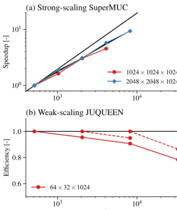
The parallel performance of MicroHH has been evaluated in strong- (cases/strongscaling) and weak-scaling (cases/weakscaling) experiments. The case used is di-rect numerical simulation of a buoyancy-driven atmospheric boundary layer based on van Heerwaarden et al. (2014). For each simulation in the scaling experiments, a series of time steps is performed, and the mean cost per step is calcu-lated over the series. The strong-scaling experiment has been performed on the Leibniz-Rechenzentrum der Bayerischen Akademie der Wissenschaften (LRZ)’s SuperMUC1 ma-chine (phase 1 thin node eight-core Sandy Bridge-EP Xeon E5-2680 8C, two processors per node, Infiniband FDR10 in-terconnect). In this experiment, simulations were performed on 1024×1024×1024 and 2048×2048×1024 grid points,
with the number of processes increased throughout the scal-ing experiment. The weak-scalscal-ing experiment has been per-formed on Forschungszentrum Jülich’s Juqueen2 machine (IBM PowerPC A2, 1.6 GHz, 16 cores per node, 5D Torus network, 40 GBps). In this experiment, a fixed 64×32×
1024 grid is assigned to each processor, and throughout the experiment the domain size is increased. The results of both experiments are shown in Fig. 12.
0 2 4 6 8 Area [%] 0
500 1000 1500 2000
z
[m]
(a)
Cloud Core
100×100×40 m 10×10×9.4m
298 300 302 304
θl[K]
(b)
Domain Cloud Core
8 12 16 20
qt[g kg−1]
(c)
0 1 2 3 4
w[m s−1]
(d)
Figure 10.BOMEX LES intercomparison (S03). Shown are the domain mean, and conditionally sampled cloud (ql>0) and cloud core (ql>0 andb− hbi>0) vertical profiles of(a)area coverage of cloud and cloud core,(b)liquid water potential temperature,(c)total specific
humidity, and (d)vertical velocity. The results are averaged over t=18 000–21 600 s. The shaded area denotes the mean ±1 standard deviation of the participating models from S03; the solid and dashed lines the results from MicroHH, using the original (solid) and a higher-resolution (dashed) setup.
263 264 265 266 267
hθi[K]
0 50 100 150 200 250 300
z
[
m
]
(a)
∆=2.00 m ∆=6.25 m
0 2 4 6 8 10
hui[m s−1]
0 50 100 150 200 250 300
z
[
m
]
(b)
0 1 2 3 4 5 6 7 8 9 Time [h] 0
50 100 150 200 250
zABL
[m]
(c)
0 1 2 3 4 5 6 7 8 9 Time [h] 0.0
0.1 0.2 0.3 0.4 0.5
u∗
[m
s
−
1]
(d)
Figure 11. GABLS1 LES intercomparison (Beare et al., 2006). Shown are the vertical profiles of(a)potential temperature and (b) u component of the velocity, and time series of the(c)boundary layer depth and(d)surface friction velocity. The shaded areas show the range
in the results from the models that participated in the Beare et al. (2006) study. The dotted black lines show the initial conditions.
The strong-scaling experiment shows that increasing the number of processors leads to faster simulations. The speedup is initially close to linear, but each consecutive in-crease in the number of cores makes the model less efficient. Based on these results, we conclude that for the chosen test case and for the used supercomputers, a work load of ap-proximately 2×10⁶grid points per core is the best balance
between speed and computational efficiency.
The weak scaling shows almost 90 % efficiency going from 512 to 8192 cores; beyond that, the scaling falls off to 80 %. This can be explained by physical properties of the ma-chine; beyond 8192 cores, a simulation no longer fits on one midplane (a physical unit consisting of 8192 cores), leading to slower communication.
10.2 Performance GPU (CUDA) implementation The GPU implementation of MicroHH allows for fast simu-lations on a single device. The current state-of-the-art GPUs
feature 12 GB of memory; thus, simulations of maximally 512×512×512 grid points of a flow with three velocity
com-ponents, pressure, two scratch fields for temporary storage, and a single scalar fit in memory. Within this experiment, we compare thus GPU simulations that do not need communica-tion against CPU simulacommunica-tions that require communicacommunica-tion be-tween cores and nodes. The reason for doing so is that nearly all of the simulations of the presented results in Sects. 8 and 9 fit within the memory of a single GPU.