R E S E A R C H
Open Access
Comparison of two projection methods for
the solution of frictional contact problems
Shougui Zhang
1*and Ruisheng Ran
2*Correspondence:
[email protected] 1School of Mathematical Sciences,
Chongqing Normal University, Chongqing, P.R. China Full list of author information is available at the end of the article
Abstract
Frictional contact problems in linear elasticity are considered in this paper. The contact constraint is imposed in the weak sense using the fixed point method, which leads to a variational equation problem. For solving such a nonlinear variational problem, we study two projection methods using different self-adaptive rules. Based on the self-adaptive projection method, we propose a modified self-adaptive rule which is more effective to update the parameter. The methods can be implemented easily in conjunction with the boundary element method for the solution. Numerical experiments are reported to illustrate theoretical results.
Keywords: Frictional contact problem; Variational inequality; Projection method; Self-adaptive rule; Boundary element
1 Introduction
Frictional contact phenomena among deformable bodies or between deformable and rigid bodies abound in industry and daily life; they play an important role in many fields of solid mechanics [1,2]. Because of the nonlinearity, the exact solution is difficult to be obtained. Therefore, a considerable effort has been made in modeling and numerical simulations of contact processes. Most of the time, the mathematical formulation of the frictional con-tact problem is reformulated as a minimization problem or a variational inequality of the second kind. Theory of contact problems and their numerical approximations has been extensively developed during the past decades [3–10]. Among the most popular methods we mention smooth Newton methods and projection methods. Although the semi-smooth Newton method is well known as the local superlinear convergence for nonlinear problems, this method converges fast only if the penalty parameter of this method is big enough, which may result in a badly conditioned problem; while the projection method with a fixed penalty parameter will be depredated significantly if the parameter is either too small or too large. Therefore, the convergence speed of these methods is sensitive to the choice of parameters. In this paper, we study the numerical solutions of frictional con-tact problems using the projection method with two self-adaptive rules for the parameter. The first method, called the self-adaptive projection method in this paper, is applica-ble for solving monotone variational inequalities of the first kind [9,11–13]. Using the equivalence between the frictional contact problem and a variational formulation with a projection fixed point problem [14–16], our method formulates the contact boundary
condition into a sequence of Robin boundary conditions. We prove the unconditional con-vergence in function spaces. The main advantage of the method is that, as compared with other methods, there is a combination of the projection method and the self-adaptive rule which uses iterative functions to update the parameter automatically.
The second method, called the modified self-adaptive projection method in this pa-per, is based on the adaptive projection method. This method uses a modified self-adaptive rule to better adjust the parameter and accelerate the convergence speed of the method, for any initial function. In addition, we note that the proof of the self-adaptive projection method for frictional contact problems can be easily extended to the modified self-adaptive projection method as well.
In these two methods, the key unknowns of frictional contact problems are displace-ment and stress on the contact boundary, which are considered primary variables and can be related in a linear system by the boundary element method (BEM) [9,10,17,18]. Be-sides, the BEM significantly reduces expense mesh generation because the formulation of the problem is concluded to the boundary of the domain. Therefore the BEM is a natural numerical tool for the solution of frictional contact problems. In this paper, we apply pro-jection methods combined with the BEM for the numerical solution of frictional contact problems.
The rest of the paper is organized as follows. First, we introduce the variational for-mulation of the classical frictional contact problem via a projection fixed point problem. Section3presents the self-adaptive projection method and the convergence analysis. Sec-tion4describes the implementation detail of the two self-adaptive rules and the boundary element approximation for the method. In Sect.5, we give some numerical results that confirm our theoretical findings. In particular, we show that the modified self-adaptive projection method has better convergence speed and stability for all parameters. Finally, Sect.6concludes the paper with some remarks.
2 Setting of the problem
We consider the classical frictional contact problem with a rigid foundation. LetΩ be an open and bounded domain inR2, with a Lipschitz boundaryΓ =∂Ω. The boundary
Γ is partitioned as three mutually disjoint parts ΓD,ΓN, andΓC=∅, where Dirichlet, Neumann, and frictional contact boundary conditions are prescribed. For simplicity, we assume that there are no volume forces acting on the body. We use n and t to denote the outward normal and tangential vectors ofΓ, respectively. For given boundary tractiontˆ∈ (L2(Γ
N))2and obstacleg∈L2(ΓC) withg> 0, the problem is to determine the displacement
usuch that
⎧ ⎪ ⎪ ⎪ ⎨ ⎪ ⎪ ⎪ ⎩
divσ(u) = 0 inΩ, (2.1)
u= 0 onΓD, (2.2)
σ(u)n =ˆt onΓN, (2.3)
un= 0 onΓC, (2.4)
and the following friction condition onΓC
if ut= 0 then|σt(u)| ≤g, (2.5)
whereutandσtare the tangential contact displacement and the tangential contact trac-tion, respectively. In this paper, we adopt the following decomposition for the displace-ment and the stress vector fields:
u=unn+ ut and σ(u)n =σn(u)n +σt(u).
Let us introduce the following Hilbert space:
V:=v∈H1(Ω)2, v|ΓD= 0,un|ΓC= 0,
and notations
a(u, v) :=
Ω
σ(u) :(v)dx,
j(v) :=
ΓC
g|vt|dsx,
L(v) :=
ΓN ˆ
t(x)·v(x)dsx.
Problem (2.1)–(2.6) is then equivalent to the following variational inequality of the second kind:
⎧ ⎨ ⎩
Find u∈Vsatisfying
a(u, v – u) +j(u) –j(v)≥L(v – u), ∀v∈V, (2.7)
or a convex minimization problem
⎧ ⎨ ⎩
Find u∈Vsuch that
J(u) =minv∈VJ(v) :=12a(v, v) –L(v) +j(v).
(2.8)
It follows from the theory of variational inequalities that problem (2.7), or equivalently (2.8), admits a unique solution [1,2]. Let us introduce a projection notation [x]αforα∈R+ and vector x∈R2
[x]α:= ⎧ ⎨ ⎩
x if|x| ≤α,
α|xx| otherwise.
Then we have the next result for the frictional boundary condition, which has been pointed out in [15].
Lemma 2.1 For allρ> 0,the frictional contact condition(2.5)–(2.6)onΓCis equivalent
to
σt(u) +
ρut–σt(u)
Now, we define the following residual function:
Rρ(ut,σt) =σt+ [ρut–σt]g onΓC. (2.10)
As a result, the nonsmooth projection equation (2.9) can be rewritten asRρ(ut,σt) = 0. Then, we propose a new equivalent formulation for the frictional boundary condition (2.5)–(2.6). For givenω= 0,Rρ(ut,σt) = 0 can be written in the following form:
σt+ρut=σt+ρut–ωRρ(ut,σt). (2.11)
Next, we apply the Green formula to (2.1)–(2.6) and obtain the variational formulation
a(u,v) –
ΓC
σt·vtdsx=L(v) ∀v∈V. (2.12)
Consequently, we obtain the following variational and projection formulations for the fric-tional contact problem (2.1)–(2.6):
⎧ ⎨ ⎩
a(u,v) –Γ
Cσt·vtdsx=L(v) ∀v∈V, σt+ρut=σt+ρut–ωRρ(ut,σt) onΓC.
(2.13)
Using this equivalent formulation, we can suggest a self-adaptive projection method for the frictional contact problem in the next section.
3 Self-adaptive projection method
In order to solve problem (2.13), we rewrite (2.11) as the following Robin iterative scheme as in [9–13]:
σt(k+1)+ρu(tk+1)=σt(k)+ρu(tk)–ωRρ
u(tk),σ(tk) onΓC. (3.1)
Then we obtain the projection method for the numerical solution of the frictional contact problem. In this method, there are two parametersω∈(0, 2) andρ> 0 which affect the convergence speed. We note that the good parameterωshould be less than and close to 2 [9–11]. Although the method converges for any fixed parameterρ> 0, the efficiency of the method depends on the parameterρheavily.
Here, we propose a projection method with a self-adaptive variable sequence of param-eters{ρk}[9,10]. In the following we need a nonnegative sequence{sk}satisfying
+∞
k=0
sk< +∞.
Now, we present the following self-adaptive projection method for the frictional contact problem.
Algorithm 1
Step 1: ComputeRρk(u(tk),σ(tk))according to (2.10). Step 2: Find(u(k+1),σ(k+1))such that
⎧ ⎪ ⎨ ⎪ ⎩
a(u(k+1),v) –
ΓCσ
(k+1)
t ·vtdsx=L(v) ∀v∈V, (3.2)
σ(tk+1)+ρku(tk+1)=σ
(k)
t +ρku(tk)–ωRρk(u
(k)
t ,σ
(k)
t ) onΓC. (3.3)
Step 3: Use a self-adaptive rule to update the parameterρk+1satisfying
1 1 +sk
ρk≤ρk+1≤(1 +sk)ρk. (3.4)
Step 4: Stop if some given stopping criterion is satisfied, else setk:=k+ 1and go to Step 1.
Letu∗andσ∗denote the solution of the frictional contact problem and the correspond-ing contact traction on the boundaryΓ, respectively. In order to establish the convergence analysis of the projection method, we have to consider preliminary results presented in the form of two lemmas.
Lemma 3.1 If the sequence{sk}satisfies sk≥0and
+∞
k=0
sk< +∞,then
+∞
k=0
(1 +sk) < +∞.
Lemma 3.2 Let (u(k),σ(k)) be the sequence generated by the self-adaptive projection
method,we have
σ(tk+1)–σ∗t +ρk
u(tk+1)–u∗t 2Γ
C
≤ σ(tk)–σ∗t +ρk
u(tk)–u∗t 2Γ
C– 2ωρk
ΓC
σt(k)–σ∗t ·ut(k)–u∗t dsx. (3.5)
Lemma3.1is obvious and Lemma3.2can refer to Theorem 3.3 in [10]. We donate
Cs:=
+∞
k=0
(1 +sk).
Consequently, it follows from Step 3 in Algorithm1that the parameterρk∈[C1sρ0,Csρ0]
is bounded. Let
ρL:=inf{ρk}+k=0∞, ρU:=sup{ρk}+k=0∞.
Then, we can prove the following convergence theorem.
Theorem 3.1 Let{(u(k),σ(k))} be the sequence generated by the self-adaptive projection
method,thenu(k)converges tou∗inVandσ(k)converges toσ∗in(L2(Γ))2.
Proof Note thatu(k)andu∗satisfy the same boundary conditions onΓ
DandΓN. We apply the Green formula to (2.1)–(2.6) and useu(nk)=u∗n= 0, it follows that
ΓC
=
ΓC
σ(tk)–σ∗t ·u(tk)–u∗t dsx
=au(k)– u∗, u(k)– u∗ ≥0. (3.6)
Since 0 <ρk+1≤(1 +sk)ρk, we use (3.5) and (3.6) and have
σ(tk+1)–σ∗t +ρk+1
u(tk+1)–u∗t 2Γ
C
≤(1 +sk)2 σt(k+1)–σ∗t+ρk
u(tk+1)–u∗t 2Γ
C
≤(1 +sk)2 σt(k)–σ∗t +ρk
u(tk)–u∗t 2Γ
C
– 2ωρk(1 +sk)2
ΓC
σ(tk)–σ∗t ·u(tk)–u∗t dsx ≤(1 +sk)2 σt(k)–σ∗t +ρk
u(tk)–u∗t
– 2ωρk
ΓC
σ(tk)–σ∗t ·u(tk)–u∗t dsx.
Then the following estimation is obtained by usingξk:= 2sk+s2k:
σ(tk+1)–σ∗t +ρk+1
u(tk+1)–u∗t 2Γ
C
≤(1 +ξk) σt(k)–σ∗t+ρk
u(tk)–u∗t 2Γ
C
– 2ωρk
ΓC
σt(k)–σ∗t ·ut(k)–u∗t dsx. (3.7)
From Lemma3.1, we have+k=0∞ξk< +∞and +∞
k=0(1 +ξk) < +∞. We introduce the fol-lowing notations:
C0:= +∞
k=0
ξk, Cp:=
+∞
k=0
(1 +ξk),
δ(uk):=u(k)–u∗, δ(ukt):=u
(k)
t –u∗t,
δσ(k):=σ(k)–σ∗, δσ(kt):=σ(tk)–σ∗t.
Thenδ(uk),δu(kt)∈Vandδσ(k),δ(σkt)∈(L2(ΓC))2. From (3.5) we have
ΓC
δσ(kt)·δu(kt)dsx=a
δ(uk),δ(uk) ≥α δ(uk) 2V, (3.8)
whereα> 0. Combining (3.7) and (3.8) we get
δ(σkt+1)+ρk+1δ(ukt+1)
2
ΓC≤(1 +ξk) δ
(k)
σt +ρ
(k) 2 δ(ukt)
2 ΓC ≤ k i=0
(1 +ξi) δ(0)σt+ρ0δ
(0)
ut
2
ΓC
≤Cp δ(0)σt+ρ0δ
(0)
ut
2
Therefore, there exists a constant C > 0 such that
δ(σk) t +ρkδ
(k)
ut
2
ΓC≤C, ∀k≥0. (3.9)
Consequently, both sequences{u(tk)}and{σ(tk)}are bounded. From (3.7), we also have
2ω +∞ k=0 ρk ΓC
σ(tk)–σ∗t ·u(tk)–u∗t dsx
≤ δ(0)σt +ρ0δ0)ut
2
ΓC+
+∞
k=0
ξk δ(σkt)+ρkδ(ukt)
2
ΓC. (3.10)
We use (3.8), (3.9), and (3.10) and obtain
∞
k=0
δ(uk) 2V
≤(2ωαρL)–1( δ(0)σt +ρ0δ
0)
ut
2
ΓC+
+∞
k=0
ξk δ(σk) t +ρkδ
(k)
ut
2
ΓC
≤(2ωαρL)–1
C+C
+∞
k=0
ξk
≤(2ωαρL)–1(1 +C0)C.
Hence, we have
lim k→∞ δ
(k)
u 2V= 0,
which means thatu(k)converges tou∗inV. From Step 2 of Algorithm1and Lebesgue’s
bounded convergence theorem it follows thatσ(k)converges toσ∗inL2(ΓC) ask→ ∞.
4 Implementation details of the proposed method
Consider that our method generates a sequence of well-posed variational problems with the common boundary condition, we can easily obtain their numerical solutions. In this section, we describe the details of the method numerically.
4.1 The self-adaptive rule
Using the method developed in [9–13], we first suggest a simple rule to adjust the variable parameterρkfor Step 3 of the self-adaptive projection method. Note that the sequence {(u(k),σ(k))}generated by Algorithm1satisfies (3.5) and (3.8), we obtain
σ(tk+1)–σ∗t +ρk
u(tk+1)–u∗t 2Γ
C≤ σ
(k)
t –σ∗t +ρk
u(tk)–u∗t 2Γ
C.
For the convergence speed of the method, we hope that
Using this idea, we update the parameterρkas follows. For a given positive constantτ, if
ρk u(tk+1)–u(tk) ΓC> (1 +τ) σ(tk+1)–σ(tk) ΓC,
we decreaseρkin the next iteration; conversely, we increaseρkwhen
ρk u(tk+1)–u(tk) ΓC< 1 1 +τ σ
(k+1)
t –σ
(k)
t ΓC.
Let
wk=
σ(tk+1)–σ(tk) ΓC
u(tk+1)–u(tk) ΓC,
we obtain the parameterρk+1according to the following self-adaptive rule:
ρk+1=
⎧ ⎪ ⎪ ⎨ ⎪ ⎪ ⎩
(1 +sk)ρk ifwk> (1 +τ)ρk,
1
1+skρk ifwk< ρk
1+τ,
ρk otherwise,
(4.2)
where the nonnegative sequence{sk}is generated by
sk= ⎧ ⎪ ⎪ ⎨ ⎪ ⎪ ⎩
τ ifck<ck+1andck+1≤cmax,
1
(ck+1–cmax)2 ifck<ck+1andck+1>cmax,
0 otherwise.
Let ckbe the change times of{ρk}, i.e.,
c0= 0, ck+1=
⎧ ⎨ ⎩
ck if 1+1τ ≤wk≤1 +τ,
ck+ 1 otherwise.
For a given constant integer cmax> 0, it follows that the sequence{sk}satisfies Lemma3.1 automatically.
4.2 The modified self-adaptive rule
Following the above self-adaptive rule, we use the same way to chooseρk+1whenwk> (1 + τ)ρkandwk<1+ρkτ. Different from the self-adaptive rule for the case
ρk
1+τ ≤wk≤(1 +τ)ρk, we give a new rule to adjustρk+1as follows. From (4.1) we have
ρk=
σ(tk+1)–σ(tk) ΓC
ut(k+1)–ut(k) ΓC =wk,
then we useρk+1=wkto replaceρk+1=ρk. Consequently, we obtain the following modified self-adaptive rule:
ρk+1=
⎧ ⎪ ⎪ ⎨ ⎪ ⎪ ⎩
(1 +sk)ρk ifwk> (1 +τ)ρk,
1
1+skρk ifwk< ρk
1+τ,
wk otherwise.
Obviously,ρk+1by using the modified self-adaptive rule also satisfies (3.4). Furthermore,
this rule is more flexible to choose a proper parameter and improve the performance of the self-adaptive rule.
4.3 Boundary element discrete form
Problem (3.2)–(3.3) is the variational formulation of the following linear elasticity prob-lem: ⎧ ⎪ ⎪ ⎪ ⎪ ⎪ ⎪ ⎨ ⎪ ⎪ ⎪ ⎪ ⎪ ⎪ ⎩
divσ(u(k+1)) = 0 inΩ, (4.4)
u(k+1)= 0 onΓ
D, (4.5)
Tu(k+1)=ˆt onΓ
N, (4.6)
u(nk+1)= 0 onΓC, (4.7)
σt(k+1)+ρku(tk+1)=σ(tk)+ρkut(k)–ωRρk(u(tk),σ(tk)) onΓC. (4.8) Since the main iterative scheme (4.8) is in the boundary of the domain, the BEM is more appropriate for the methods [9,10,17,18].
The solutionuof problem (4.4)–(4.8) can be represented as theBetti–Somigliana rep-resentation formula
u(y) =
Γ
G(x,y)Tu(x)dsx–
Γ
TxG(x,y) Tu(x)dsx, (4.9)
where thex inTxG(x,y) denotes differentiations in (4.6) with respect to the variablex, andG(x,y) is the fundamental solution of the two-dimensional Lamé equation. The dis-placementsuand tractionsTusatisfy the boundary integral equation
1 2u(y) =
Γ
G(x,y)Tu(x)dsx–
Γ
TxG(x,y)Tu(x)dsx ∀y∈Γ. (4.10)
The boundaryΓis approximated byNstraight line elements. We use constant boundary elements, and the nodes are located in the middle of each element. Using functionsu(tk)and σ(tk), we obtain the projection residual functionRρk(u
(k)
t ,σ(tk)) point-wise on nodes element by element alongΓC. We applyun= 0 and the Robin boundary condition
σt(k+1)=σ(tk)+ρut(k)–u(tk+1) –ωRρk
u(tk),σ(tk) (4.11)
to (4.10) to eliminateσn(k+1)and obtain the corresponding discrete form atx∈ΓC
u(k+1)(y
i)
2 +
ΓC
u(k+1)(yj)TxG(x,yi)Tdsx+
ΓC
ρku(tk+1)(xj)G(x,yi)dsx
=
ΓC
σt(k)(xj) +ρkut(k)(xj) –ωRρk
u(tk)(xj),σ(tk)(xj) G(x,yi)dsx yi∈Γ. (4.12)
On the boundaryΓD∪ΓN, the discrete form of the boundary integral equation reads as follows:
u(k+1)(y
i)
2 +
ΓD∪ΓN
u(k+1)(xj)TxG(x,y))Tdsx
=
ΓD∪ΓN
Using all the boundary conditions (4.5)–(4.8), we can solve the linear systems (4.12) and (4.13) to obtain both displacementu(k+1)and stressσ(k+1)at the nodes onΓ. So that we can
reset the parameter and the Robin boundary condition onΓCaccording to the method.
5 Numerical experiments
In this section, we present some numerical results to compare the performance of the projection method with different self-adaptive rules. In all tests, we takeω= 1.8 andτ= 2,
cmax= 10 for our methods. Here, we choose
u(k+1)–u(k) L2(Γ
C)+σ (k+1)
t –σ(tk) L2(ΓC)
u(k+1)
L2(ΓC)+σ
(k+1)
t L2(ΓC)
≤10–6 as a
stopping criterion and use Matlab codes for our methods.
5.1 Example 1
We consider an elastic bodyΩ= (0, 8)×(0, 4). The bottom of the rectangle is in contact with a rigid foundation and the frictional contact part of the boundary isΓC= (0, 8)× {0}. On the partΓD= (0, 8)× {4}the body is clamped. The Neumann boundary condition is given byˆt= (400, 0)on{0} ×(0, 4), andˆt= 0 on the rest ofΓN. The elasticity parame-ters are chosen to be Young’s modulusE= 10,000 and Poisson’s ratiov= 0.3, the friction coefficient isg= 150 daN/mm2onΓ
C.
First we apply our methods to this problem with initial parameterρ= 1 and step size
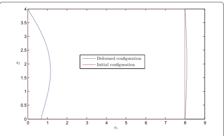
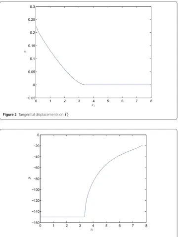
h= 0.05, and the initial and deformed configurations of the body are shown in Fig.1. On
ΓC, the tangential displacement and traction are depicted in Figs.2and3, respectively. We note thatΓCis divided into a slip part and a stick part with a transition point from slip to stick near (3.3, 0). It can be seen that our results are in a good agreement with those in Ref. [5].
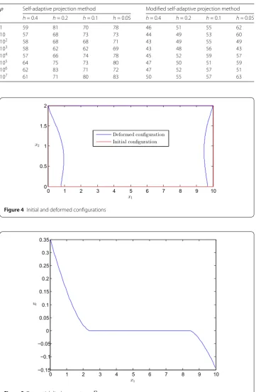
Here, we test the problem with different initial positive parametersρand mesh sizesh. In Table1, we give the number of iterations for the convergence of the self-adaptive pro-jection and modified self-adaptive propro-jection methods with rules (4.2) and (4.3), respec-tively. According to these numerical results, as expected, all parametersρdo not have a significant effect on the number of iterations for each method. Moreover, the number of
Figure 2Tangential displacements onΓC
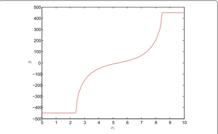
Figure 3Tangential tractions onΓC
iterations for the method depends only weakly onh. In particular, the number of itera-tions of modified self-adaptive projection method is less than the self-adaptive projection method.
5.2 Example 2
Table 1 Number of iterations for each method
ρ Self-adaptive projection method Modified self-adaptive projection method
h= 0.4 h= 0.2 h= 0.1 h= 0.05 h= 0.4 h= 0.2 h= 0.1 h= 0.05
1 59 81 70 78 46 51 55 62
10 57 68 73 73 44 49 53 60
102 58 68 68 71 43 49 55 49
103 58 62 62 69 43 48 56 43
104 57 66 74 78 45 52 59 57
105 64 75 73 80 47 50 51 59
106 62 83 71 72 47 52 57 51
107 61 71 80 83 50 55 57 63
Figure 4Initial and deformed configurations
Figure 5Tangential displacements onΓC
We chooseρ= 1 andh= 0.05 again and apply our method to this problem. Figure4
Figure 6Tangential tractions onΓC
Table 2 Number of iterations for each method
ρ Self-adaptive projection method Modified self-adaptive projection method
h= 0.4 h= 0.2 h= 0.1 h= 0.05 h= 0.4 h= 0.2 h= 0.1 h= 0.05
1 53 64 71 55 43 47 50 51
10 49 62 72 62 42 45 48 38
102 50 55 59 55 40 44 47 49
103 47 58 64 57 39 42 45 46
104 49 59 71 63 41 44 48 48
105 49 57 61 54 42 44 46 48
106 53 63 70 54 45 46 49 49
107 54 65 74 67 46 48 52 54
(2.4, 0) and (8.4, 0). It can be observed that our results are in agreement with conditions (2.5) and (2.6) again. We also investigate the convergence behavior of our method for this example. Table2displays the number of iterations with respect to the parameterρand the mesh sizeh. As in the previous example, our modified self-adaptive projection method is better than the self-adaptive projection method, because this method accelerates the con-vergence speed.
6 Conclusion
Acknowledgements
Not applicable.
Funding
This work is funded by the National Natural Science Foundation Project of CQ CSTC of China (Grant nos.
cstc2017jcyjAX0316 and cstc2016jcyjA0419) and the School Fund Project of Chongqing Normal University (CQNU) (Grant no. 16XZH07).
Availability of data and materials
All data are fully available without restriction.
Competing interests
The authors declare that they have no competing interests.
Authors’ contributions
All authors equally have made contributions. All authors read and approved the final manuscript.
Author details
1School of Mathematical Sciences, Chongqing Normal University, Chongqing, P.R. China.2College of Computer and
Information Science, Chongqing Normal University, Chongqing, P.R. China.
Publisher’s Note
Springer Nature remains neutral with regard to jurisdictional claims in published maps and institutional affiliations.
Received: 26 September 2018 Accepted: 7 April 2019 References
1. Glowinski, R.: Numerical Methods for Nonlinear Variational Problems. Springer, Berlin (2008) 2. Han, W.M.: A Posteriori Error Analysis Via Duality Theory. Springer, New York (2005)
3. Stadler, G.: Semismooth Newton and augmented Lagrangian methods for a simplified friction problem. SIAM J. Optim.15, 39–62 (2004)
4. De Los Reyes, J.C., Hintermüller, M.: A duality based semismooth Newton framework for solving variational inequalities of the second kind. Interfaces Free Bound.13, 437–462 (2011)
5. Bostan, V., Han, W.M.: A posteriori error analysis for finite element solutions of a frictional contact problem. Comput. Methods Appl. Mech. Eng.195, 1252–1274 (2006)
6. Denkowski, Z., Migórski, S., Ochal, A.: A class of optimal control problems for piezoelectric frictional contact models. Nonlinear Anal., Real World Appl.12, 1883–1895 (2011)
7. Touzaline, A.: Optimal control of a frictional contact problem. Acta Math. Appl. Sin. Engl. Ser.31, 991–1000 (2015) 8. Wang, F., Han, W.M., Cheng, X.L.: Discontinuous Galerkin methods for solving a quasistatic contact problem. Numer.
Math.126, 771–800 (2014)
9. Zhang, S.G., Li, X.L.: A self-adaptive projection method for contact problems with the BEM. Appl. Math. Model.55, 145–159 (2018)
10. Zhang, S.G., Li, X.L., Ran, R.S.: Self-adaptive projection and boundary element methods for contact problems with Tresca friction. Commun. Nonlinear Sci. Numer. Simul.68, 72–85 (2019)
11. He, B.S., Liao, L.Z., Wang, S.L.: Self-adaptive operator splitting methods for monotone variational inequalities. Numer. Math.94, 715–737 (2003)
12. Bnouhachem, A.: An inexact implicit method for general mixed variational inequalities. J. Comput. Appl. Math.200, 417–426 (2007)
13. Ge, Z.L., Han, D.R.: Self-adaptive implicit methods for monotone variant variational inequalities. J. Inequal. Appl.2009, Article ID 458134 (2009)
14. Chouly, F.: A Nitsche-based method for unilateral contact problems: numerical analysis. SIAM J. Numer. Anal.51, 1295–1307 (2013)
15. Chouly, F.: An adaptation of Nitsche’s method to the Tresca friction problem. J. Math. Anal. Appl.411, 329–339 (2014) 16. Zhang, S.G., Li, X.L.: An augmented Lagrangian method for the Signorini boundary value problem with BEM. Bound.
Value Probl.2016, 62 (2016)
17. Hsiao, G.C., Wendland, W.L.: Boundary Integral Equations. Springer, Berlin (2008)