*Corr. Author’s Address: LMT-Cachan ENS Cachan/CNRS/Paris 6 University, PRES UniverSud Paris 61 avenue du President Wilson,
F-94230 Cachan, France, [email protected] 307
Strojniški vestnik - Journal of Mechanical Engineering 60(2014)5, 307-313 Received for review: 2013-10-16 © 2014 Journal of Mechanical Engineering. All rights reserved. Received revised form: 2014-01-17 DOI:10.5545/sv-jme.2014.1834 Special Issue, Original Scientific Paper Accepted for publication: 2014-04-01
0 INTRODUCTION
The prediction of the frequency responses of complex systems in frequency bands is required in many industrial applications, like car or aerospace acoustics. Since the complex matrix of the finite element is wavenumber dependent, the computation of the vibrational solution often involves the resolution of the problem at each frequency of the frequency band, then leading to a prohibitive computational cost. This is particularly true in the mid-frequency regime, where the solutions are sensitive to frequency, requiring a very refined frequency discretization. The definition of advanced numerical strategies for predicting the acoustic response of complex systems in the mid-frequency ranges is the subject of this work. It uses the combination of the variational theory of complex rays (VTCR) [1] and the proper generalized decomposition (PGD) [2].
The VTCR has been introduced in [3] and is dedicated to the resolution of mid-frequency problems. It is a Trefftz method which uses oscillating waves to expand the field variables. It is based on an original variational formulation designed such that the approximations within the substructures are totally independent, which means that any kind of approximation can be used, even those which have a strong physical content, giving to the strategy a strong flexibility, and hence efficiency. It has already been developed for plates, [4] shells [5] acoustics in 2D [6] or 3D [1], vibration problems, and also for transient applications [7]. It distinguishes itself from the other Trefftz techniques [8] to [13] by the type of selected
shape functions and the treatment of the boundary conditions.
The PGD is a model order reduction technique. Introduced in [2], it has already been successfully utilized for the resolution of multi-parametric problems (problems which depend on many parameters such as the space and time problems, or the space and uncertain problems, etc.) [14] to [16]. The resolution of the vibration problem (with the VTCR) at many frequencies is such a multi-parametric problem. Therefore, a combination of PGD and the VTCR is an obvious choice to handle frequency problems in medium frequency bands.
The VTCR has already been extended to frequency band applications [17] and [18]. In these works, the authors proposed new algorithms for the calculation of multiple frequency solution, either by using a set of parameters to derive a discrete approximation of the frequency-dependent quantities within the VTCR matrix, or by expanding the VTCR matrix into series with respect to the frequency. In this work, we propose a new path to determine the frequency response of a system at many frequencies. It is based on a combination of the VTCR, used to find the solution of the vibration problem at a fixed frequency, and the PGD, used to find the best separated variable representation of this solution over a frequency band. Power type algorithms are proposed to find it in an efficient way. A 2-D numerical illustration on a car cavity is proposed to see the benefits of such an approach.
PGD-VTCR: A Reduced Order Model Technique
to Solve Medium Frequency Broad Band Problems
on Complex Acoustical Systems
Barbarulo, A. – Riou, H. – Kovalevsky. L. – Ladeveze, P.Andrea Barbarulo1,* – Hervé Riou1 – Louis Kovalevsky2 – Pierre Ladeveze1
1 LMT-Cachan, ENS Cachan, France
2 University of Cambridge, Engineering department, United Kingdom
The calculation of vibrational responses of complex systems on frequency bands appears to be more and more important in engineering simulation. This is particularly true in the medium frequency regime where the solution is very sensitive to the frequency. In this work, we propose a new path to determine the frequency response of a system at many frequencies. It is based on the variational theory of complex rays (VTCR), a mid frequency dedicated numerical strategy, and the proper generalized decomposition (PGD), a model order reduction technique. The VTCR enables one to model the problem thanks to the use of waves, and the PGD expands the VTCR approximation over the frequency band through a separated variable representation. This strategy is illustrated on a 2-D acoustic car cavity example.
Strojniški vestnik - Journal of Mechanical Engineering 60(2014)5, 307-313
308 Barbarulo, A. – Riou, H. – Kovalevsky. L. – Ladeveze, P.
1 THE REFERENCE ACOUSTICAL PROBLEM TO SOLVE
Consider a fluid comprised in a bounded domain Ω. This fluid is characterized by its speed of sound
c0 and its density ρ0. We study the steady-state
vibration response of the fluid in the frequency band
I = [ω0 – Δω/2; ω0 + Δω/2] where ω0 is the central
frequency and Δω the frequency bandwidth. The reference problem to solve is: find the pressure
p(x, ω), (x, ω) ∈ Ω×I, such that:
∆p k p I
p p I
L p v I
p ZL p h
d p
v d v
v d
+ = ×
= ∂ ×
( )
= ∂ ×−
( )
=2 0 over
over over ov Ω Ω Ω eer∂ZΩ×I
. (1)
In Eq. (1), k = (1 – iη) ω / c0 is the wave number
(η is the absorption coefficient), pd is a prescribed
pressure, Z is a prescribed velocity, hd a given
impedance and a given function. The operator Lv is such that Lv(p) = (i/ρ0ω) (∂p/∂n). ∂pΩ, ∂vΩ and ∂zΩ are the parts of the boundary of Ω where the pressure, the velocity and the Robin conditions are prescribed. The uniqueness of the solution is ensured by a strictly positive η. If Ω is paritioned in nel non-overlapping
elements Ωe, one must also consider the additional
continuity equation at the common boundary Γe,e' = Ωe ∩ Ωe' :
p p
L pv ee L pve e e e e e
− =
( )
+( )
= ' ' ' ' 0 0 along along Γ Γ ,, . (2)
2 THE VTCR FORMULATION OF THE REFERENCE PROBLEM
The VTCR forumulation of an acoustic problem can be found in [6]. It necessitates the definition of the space of functions which exactly satisfy the governing equation (first equation of Eq. (1)) over the subdomains Ωe:
Se=
{
pe;∆p k pe+ 2 e=0 overΩe×I}
. (3) Problem (Eqs. (1) and (2)) can then be formulated as: find(
p p1, 2,...,pnel)
∈ ×S S1 2× ×... Snel such that:e e de v e
e e v e de
e e v e
p p L p dS
p L p v dS
p ZL p
∑∫
∑∫
∑∫
−(
) (
)
+ +(
( )
−)
+ + −( )
− δ δhh L p dS
p p L p L p dS
d v e
e e e e e v e v e
(
)
(
)
+ +(
−) (
(
)
−(
)
)
+ + >∑ ∫
δ δ δ 1 2 1 2 ,' ' 'ee e e e e v e v e
p p L p L p dS
p p S
,
,...,
'> ' '
∑ ∫
(
+) ( )
(
+( )
)
== ∀
(
)
∈δ δ
δ δ
0 × ×... S ,
e e v e de
e e v e
p L p v dS
p ZL p
∑∫
∑∫
+
(
( )
−)
++ −
( )
−δ
hh L p dS
p p L p L p dS
d v e
e e e e e v e v e
(
)
(
)
+ +(
−) (
(
)
−(
)
)
+ + >∑ ∫
δ δ δ 1 2 1 2 ,' ' 'ee e e e e v e v e
nel
p p L p L p dS
p p S
,
,...,
'> ' '
∑ ∫
(
+) ( )
(
+( )
)
== ∀
(
)
∈δ δ
δ δ
0 1 11× ×... Snel, (4)
where pde, vde and hde are the boundary conditions
defined in Eq. (1) but restricted to ∂Ωe. The
overline designates the complex value quantity. The equivalence between Eqs. (1) and (4) car be found in references on the VTCR. Eq. (4) can be written: find
p∈S such that:
a p p
(
,δ)
=l p( )
δ ∀δp S∈ , (5) where a and l are the bilinear and the linear part of Eq. (4).3 THE APPROXIMATED SOLUTION OF THE REFERENCE PROBLEM
The only thing to do in order to get an approximated solution of the reference problem Eqs. (1) and (2) is to satisfy Eq. (5) in a subspace Sh⊂S. As one can see,
S is defined such that the approximations in Se can be independant of one another. As a consequence, any kind of approximated solution can be selected to span
Sh, as soon as it satisfies the governing equation (first
equation of Eq. (1)) in Ωe. The VTCR approximation
uses propagating waves inside the acoutics domains, and consider all of them. For instance, in the 2-D modeling, we have:
p x
(
,ω)
∈Se⇔p x(
,ω)
=∫
Xe(
θ ω,)
e dikex θ, (6)where ke is the wavenumber of the vibration problem
in Ωe. Corresponding 3-D modeling can be found
in [1]. Xe(θ,ω) corresponds to the amplitudes of the waves, and is the unknown of the problem. Different approximations of Xe(θ,ω) can be used (see [19]). If the Fourier approximation is used, we expand Xe(θ,ω) on a Fourier series in order to define the subspace Sh:
Xe
(
θ ω,)
Xeh(
θ ω,)
=∑
Xen( )
ω einθ. (7)As a consequence, the subspace Seh is spanned by
the shape functions φ ω θ θ
en( , )x =
∫
e e din ikex and, for afixed frequency, Xeh
( )
ω are the VTCR unknownsStrojniški vestnik - Journal of Mechanical Engineering 60(2014)5, 307-313
309 PGD-VTCR: A Reduced Order Model Technique to Solve Medium Frequency Broad Band Problems on Complex Acoustical Systems
The substitution of Eqs. (6) and (7) into Eq. (5) leads to the frequency band matrix system :
K(ω) X(ω) = F(ω), (8)
where K(ω) and F(ω) are the projection of the
bilinear and the linear forms of Eq. (5) onto the space generated by the functions φen. In the following, N
will designate the size of X(ω).
4 THE COMBINATION OF THE PGD AND THE VTCR TO SOLVE THE FREQUENCY BAND PROBLEM
The problem given by Eq. (8) defined on the frequency
band I is a multiparametric problem: the solution
X(ω) contains information related to the direction
of propagation of the waves and to the frequency. Solving this problem has already be considered in previous works on the VTCR either by using a set of parameters to derive a discrete approximation of the frequency-dependent quantities within the VTCR matrix or by expanding the VTCR matrix and the right-hand side of the system into series with respect to the frequency [17] and [18]. Here, we propose a new path to solve this, based on a model order reduction technique through a separated variable representation of the physical data. Today, the common name, which designates a decomposition of the physical data in a separated representation of the variables, is the proper generalized decomposition (PGD) (see [20] for a general review on PGD). With such a decomposition, any physical variable can be decomposed into a separated variable decomposition:
u x xR uM x x u x u x
R m mR R
1,..., 1,..., 1 1 ... ,
(
)
(
)
=∑
( )
× ×( )
M being the order of the approximation. As a
consequence, the strategy used to solve Eq. (8) on I is to search the solution X(ω) in the form:
X XM X
m m
ω ω λ ω
( )
( )
=∑
( )
, (9)where Xm are constant vectors in N and λm(ω)
frequency functions in T, space of functions whose
square integration on I is finite.
Of course, neither Xm or λm(ω) are known. Then the key questions are: (i) how can we define the optimal decomposition; (ii) how can we compute it? If the solution X(ω) is known, it suffices to minimize the distance between this solution and the best approximation:
X X min X X
m M
m m
X XM N M T m M m m − = − = ∈ ∈ =
∑
∑
1 2 1 1 1 2 λ λ λ λ ,..., ,..., , (10)
according to a given norm on N and T. But here, we want to build a decomposition Eq. (8) of the solution
X(ω) without knowing this solution a priori. Notice
that neither λm nor Xm are uniquely defined, as any other decomposition which multiplies λm by a constant factor and divide Xm by the same factor works also. Therefore, without loss of generality, we can prescribe
the normalization of Xm according to the euclidean
norm on N.
In order to build the best approximation, without knowing X, let us first write the problem in a variational formulation. Solving Eq. (8) on I can be written: find X(ω) ∈ N ⊗T such that:
B X
(
( ) ( )
ω ,Y ω)
=L Y(
( )
ω)
∀Y( )
ω ∈N⊗T, (11) where,B X
(
( ) ( )
ω ,Y ω)
=∫
Y( ) ( ) ( )
ω TK ω X ω ωd and L Y(
( )
ω)
=∫
Y( ) ( )
ω TF ω ωd(the superscript T stands for the complex transpose vector definition). Moreover, let us define the inner product <<.,>> on N ⊗ T by:
<<
( )
( )
>>=( )
(
)
( )
(
( )
)
∫
λ ω γ ω γ ω ω λ ω ω X YY H X d
,
, T
(12)
where H
( )
ω =Hh( )
ω (H being the constant matrix of the mean value of K(ω) over I and h( )
ω the frequency dependent function of the mean value of the diagonal part of K(ω)). This choice provides some optimal convergence properties [21] by preserving a relation to the initial problem to solve, and moreover ensures we have the inner product separation propertyA X Y X X
B X X Y L Y
M M λ γ λ λ λ γ γ , , , .
(
)
= << >> −−
(
− +)
+( )
1 2 1
, where <.,>N is a norm on N and <.,>T a norm on T. Finally, we introduce the functional AM(X, Y ,λ ,γ) defined on
N×N × T × T by:
A X Y X X
B X X Y L Y
M M λ γ λ λ λ γ γ , , , .
(
)
= << >> −−
(
− +)
+( )
1 2
1 (13)
According to the Petrov Galerkin PGD approach introduced in [21], we define the best representation Eq. (9) of the solution of the problem Eq. (8) defined on I by the following minimax problem:
λ γ
λ γ
γ λ
M M M M Y N T X N T M
X Y
arg max min A X Y
,
, .
, ,
(
)
∈
(
)
Problem (Eq. (14)) can be interpreted as a pseudo eigen problem, corresponds to the definition of the best rank-one separated representation of X – XM–1
and is a generalization of the proper generalized decomposition (POD) [21].
According to Eq. (14), we can see that the best separated representation makes stationary the functional AM(X, Y ,λ ,γ) with respect to X, Y, λ and γ. These stationary conditions write:
B XM X Y L Y Y
M M M M N
− +
(
1 λ ,γ ')
=(
γ ')
∀ ∈' , (15)B X
(
M−1+λMXM,γ'YM)
=L Y(
γ' M)
∀ ∈γ' T, (16) B(
λMX',γM MY)
=<<λMX',λMXM >> ∀ ∈X' N,(17) B X(
λ' M,γM MY)
=<<λ'XM,λMXM >> ∀ ∈λ' T. (18) Then, according to the combination of the PGD and the VTCR, the best separated variable representation Eq. (9) of the reference problem Eqs. (1) and (2) is simply the solution of Eqs. (15) to (18).5 POWER TYPE ALGORITHM FOR THE CONSTRUCTION OF THE APPROXIMATION
We have seen that the best representation Eq. (9) of problem (Eq. (8)) defined on I must verify Eqs. (15) to (18). As these equations are coupled, a natural approach to find the solution is to build solutions
X, Y, λ and γ one after the other, which is the strategy adopted in power iterative algorithms. As a consequence, we can define the Algorithm 1, which looks at the solution of Eqs. (15) to (18):
Algorithm 1 form = 1 to Mdo Initialize λ(ω) and γ(ω) forq = 1 to Qdo
Compute Xm( )q and Ym( )q by using Eqs. (15) and (17) Normalize Xm( )q and Ym( )q and
Compute λm( )q and γm( )q by using Eqs. (16) and (18) Set
(
Xm,λm)
=(
Xm( ) ( )q ,λmq)
Compute ( )q , the distance between
(
Xm( ) ( )q ,λmq) (
and Xm( )q−1,λm( )q−1)
if ( )q <Q then
break end if end for
Set Xm = Xm–1 + λmXm
Compute m, the error between KXm and F
ifm<M then
break
end if end for
The first loop corresponds to the recursive
construction of couples (λmXm). This loop begins
with the initialization of λ(ω) and γ(ω). We always prescribe:
KXm− −F T KXm− F
(
1)
(
1−)
,as an initialization value, in order to begin the algorithm with a relation to the target problem. The second loop is the alternate construction of the pairs (Xm, λm) and (Ym, γm) and is based on a power iterative technique to find the stationary point defined by Eqs. (15) to (18). The normalization of the vectors, discussed before, is done in this loop. We introduce a stopping criteria inside the loop to see if the power iterative technique has converge or not. This criteria is based on the relative norm between the pair
Xm( ) ( )q mq Xm( )q− m( )q−
(
,λ) (
and 1,λ 1)
, over the frequencyband. If the solution at iterationis (q) is closed to
the solution at iteration (q–1), the second loop is
stopped, because the power iterative technique has converged toward the stationary point of Eqs. (15) to (18). As soon as the second loop has finished, we actualize the solution (Xm, λm). Finally, we compute the error indicator m = || KXm – F || / || F || to assess the precision of the approximation Eq. (9).
In practice, the alternate minimization procedure of the second loop converges very fast. As a consequence, we can then classically limit the number of iterations Q to 8 or 9.
6 NUMERICAL ILLUSTRATION
Consider the closed acoustic car cavity defined on Fig. 1. This cavity is filled with a fluid close to the air (ρ0 = 1.25 kg/m3, c0 = 340 m/s and η = 0.0005).
Different boundary conditions are prescribed on the boundaries of the cavity: prescribed velocity or prescribed impedance (see Fig. 1). The black zone corresponds to the measure area, where the evaluation of the acoustical energy is desired. It corresponds more or less to the zone where the hear of the driver is located.
The cavity is modeled by the VTCR with 8
Strojniški vestnik - Journal of Mechanical Engineering 60(2014)5, 307-313
311 PGD-VTCR: A Reduced Order Model Technique to Solve Medium Frequency Broad Band Problems on Complex Acoustical Systems
seen on Fig. 1 (the continuous black lines make a separation between them). In each Ωe, the VTCR uses 2Ne + 1 shape functions φen (defined in Eq. (7)) such
that the convergency criteria in [19] is respected. The considered central frequency is ω0 = 2π × 2150 rad/s
and the bandwidth is Δω = 2π × 300 rad/s. The Algorithm 1 described in Section 6 is used to get an approximated solution. The parameter (see Section 5) has been retained. For the comparison, the reference solution is given by the VTCR strategy solely, with a computation at many frequencies.
Fig. 1. Definition of the closed acoustic car cavity considered in Section 6
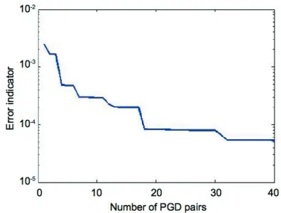
Fig. 2 shows the error indicator m defined in
Section 5 versus the number of PGD pairs (Xm, λm)
that are selected. As one can see, this error indicator decreases, which illustrates the convergence of the Algorithm 1. As m quantifies the error in the resolution of the VTCR problem (Eq. (8)) on the whole frequency band, its convergence simply tells us that the PGD-VTCR approximated solution is convergent over the whole frequency band.
Fig. 3 shows a comparison between the VTCR reference solution and the PGD-VTCR approximation at ω0 – Δω / 2, ω0 and ω0 + Δω / 2 (the middle and
the two extreme circular frequency of the frequency
band). As one can from the eye-ball norm, the solutions are very closed each time. Indeed, for each considered case, the localization of the vibrational peaks and their amplitude are the same. This illustrates that the proposed Algorithm 1 is able to recover the reference solution over the whole frequency band. This is of course in agreement with the last remark on the convergence of the error indicator, whose convergence is visible on Fig. 2: this error indicator being convergent, the solution is correct over the whole frequency band.
Fig. 2. The error indicator (see Section 5) versus the number of PGD pairs (Xm, λm) selected
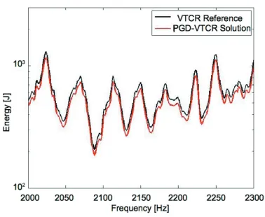
Finally, Fig. 4 depicts the acoustical energy in the measure area defined in Fig. 1, over the whole frequency band. This energy is easy to compute from the local response, which is visible on Fig. 3. Again, the comparison of this physical quantity computed by the PGD-VTCR approximation with the same quantity computed on the reference solution shows that the proposed approach is able to recover the reference solution very well, on the whole frequency band.
Fig. 4. Comparison between the solution given by the PGD approximation with (red color curve) and the VTCR reference solution (black color curve) for the example considered in Section
6 and described in Fig. 1
7 CONCLUSIONS
We proposed here a new path for solving vibration problems on frequency bands. It is based on a combination of the VTCR and the PGD. Looking for an approximation based on a separated variable decomposition solves the VTCR problem, defined on a frequency band. The best representation of such decomposition has been defined through a minimax problem, which is a generalization of the PGD. Power type algorithms have been proposed to find the solution of the minimax problem. A 2-D numerical illustration on a car cavity has been proposed to see the benefits of such an approach on complex acoustical problems. Future works will be devoted to the definition of more efficient algorithms to find a separated variable decomposition. The extension of this strategy to problems with uncertainties is also a work in progress.
8 REFERENCES
[1] Kovalevsky, L., Ladevèze, P., Riou, H., Bonnet, M. (2012). The variational theory of complex rays for three-dimensional helmholtz problems. Journal of Computational Acoustics, vol. 20, no. 4, DOI:10.1142/ S0218396X1250021X.
[2] [2] Ladevèze, P. (1999). Nonlinear Computational Structural Mechanics - New Approaches and Non-Incremental Methods of Calculation, Springer, Berlin, DOI:10.1007/978-1-4612-1432-8.
[3] Ladevèze, P. (1996). A new computational approach for structure vibrations in the medium frequency range. Comptes Rendus de l Académie des Sciences - Series IIB - Mechanics-Physics-Chemistry-Astronomy, vol. 332, p. 849-856.
[4] Rouch, P., Ladevèze, P. (2003). The variational theory of complex rays: a predictive tool for medium-frequency vibrations. Computer Methods in Applied Mechanics and Engineering, vol. 192, no. 28-30, p. 3301-3315, DOI:10.1016/S0045-7825(03)00352-9. [5] Riou, H., Ladevèze, P., Rouch, P. (2004). Extension
of the variational theory of complex rays to shells for medium- frequency vibrations. Journal of Sound and Vibration, vol. 272, no. 1-2, p. 341-360, DOI:10.1016/ S0022-460X(03)00775-2.
[6] Riou, H., Ladevèze, P., Sourcis, B. (2008). The multiscale VTCR approach applied to acoustics problems. Journal of Computational Acoustics, vol. 16, no. 4, p. 487-505, DOI:10.1142/S0218396X08003750. [7] Ladevèze, P., Chevreuil, M. (2005). A new
computational method for transient dynamics including the low-and the medium-frequency ranges. International Journal for Numerical Methods in Engineering, vol. 64, no. 4, p. 503-527, DOI:10.1002/ nme.1379.
[8] Strouboulis, T., Hidajat, R. (2006). Partition of unity method for helmholtz equation: q-convergence for plane- wave and wave-band local bases. Applications of Mathematics, vol. 51, no. 2, p. 181-204, DOI:10.1007/ s10492-006-0011-0.
[9] Cessenat, O., Despres, B. (1999). Application of an ultra weak variational formulation of elliptic pdes to the two-dimensional helmholtz problem. SIAM Journal on Numerical Analysis, vol. 35, no. 1, p. 255-299, DOI:10.1137/S0036142995285873.
[10] Monk, P., Wang, D. (1999). A least-squares method for the Helmholtz equation. Computer Methods in Applied Mechanics and Engineering, vol. 175, no. 1-2, p. 121-136, DOI:10.1016/S0045-7825(98)00326-0.
[11] Farhat, C., Harari, I., Franca, L. (2001). The discontinuous enrichment method. Computer Methods in Applied Mechanics and Engineering, vol. 190, no. 48, p. 6455-6479, DOI:10.1016/S0045-7825(01)00232-8.
[12] Perrey-Debain, E., Trevelyan, J., Bettess, P. (2004). Wave boundary elements: a theoretical overview presenting applications in scattering of short waves. Engineering Analysis with Boundary Elements, vol. 28, no. 2, p. 131-141, DOI:10.1016/S0955-7997(03)00127-9.
[13] Van Genechten, B., Atak, O., Bergen, B., Deckers, E., Jonckheere, S., Lee, J.S., Maressa, A., Vergote, K., Pluymers, B., Vandepitte, D., Desmet, W. (2012). An efficient Wave Based Method for solving Helmholtz problems in three- dimensional bounded domains. Engineering Analysis with Boundary Elements, vol. 36, no. 1, p. 63-75, DOI:10.1016/j. enganabound.2011.07.011.
Strojniški vestnik - Journal of Mechanical Engineering 60(2014)5, 307-313
313 PGD-VTCR: A Reduced Order Model Technique to Solve Medium Frequency Broad Band Problems on Complex Acoustical Systems
vol. 139, no. 3, p. 153-176, DOI:10.1016/j. jnnfm.2006.07.007.
[15] Nouy, A. (2007). A generalized spectral decomposition technique to solve a class of linear stochastic partial differential equations. Computer Methods in Applied Mechanics and Engineering, vol. 196, no. 45-48, p. 4521-4537, DOI:10.1016/j.cma.2007.05.016.
[16] Ladevèze, P., Passieux, J.C., Néron, D. (2010). The LATIN multiscale computational method and the proper generalized decomposition. Computer Methods in Applied Mechanics and Engineering, vol. 199, no. 21-22, p. 1287-1296, DOI:10.1016/j.cma.2009.06.023. [17] Ladevèze, P., Rouch, P., Riou, H., Bohineust, X.
(2003). Analysis of medium-frequency vibrations in a frequency range. Journal of Computational Acoustics, vol. 11, p. 255-284, DOI:10.1142/ S0218396X0300195X.
[18] Ladevèze, P., Riou, H. (2005). Calculation of medium-frequency vibrations over a wide frequency
range. Computer Methods in Applied Mechanics and Engineering, vol. 194, no. 27-29, p. 3167-3191, DOI:10.1016/j.cma.2004.08.009.
[19] Kovalevsky, L., Ladevèze, P., Riou, H. (2012). The Fourier version of the variational theory of complex rays for medium-frequency acoustics. Computer Methods in Applied Mechanics and Engineering, vol. 225-228, p. 142-153, DOI:10.1016/j.cma.2012.03.009. [20] Chinesta, F., Ladevèze, P., Cueto, E. (2011). A short
review on model order reduction based on proper generalized decomposition. Archives of Computational Methods in Engineering, vol. 18, no. 4, p. 395-404, DOI:10.1007/s11831-011-9064-7.