R E S E A R C H A R T I C L E
Open Access
Estimating the loss of lifetime function
using flexible parametric relative survival
models
Lasse H. Jakobsen
1,2*, Therese M.-L. Andersson
3, Jorne L. Biccler
1,2, Tarec C. El-Galaly
1,2and Martin Bøgsted
1,2Abstract
Background: Within cancer care, dynamic evaluations of the loss in expectation of life provides useful information to patients as well as physicians. The loss of lifetime function yields the conditional loss in expectation of life given survival up to a specific time point. Due to the inevitable censoring in time-to-event data, loss of lifetime estimation requires extrapolation of both the patient and general population survival function. In this context, the accuracy of different extrapolation approaches has not previously been evaluated.
Methods: The loss of lifetime function was computed by decomposing the all-cause survival function using the relative and general population survival function. To allow extrapolation, the relative survival function was fitted using existing parametric relative survival models. In addition, we introduced a novel mixture cure model suitable for extrapolation. The accuracy of the estimated loss of lifetime function using various extrapolation approaches was assessed in a simulation study and by data from the Danish Cancer Registry where complete follow-up was available. In addition, we illustrated the proposed methodology by analyzing recent data from the Danish Lymphoma Registry. Results: No uniformly superior extrapolation method was found, but flexible parametric mixture cure models and flexible parametric relative survival models seemed to be suitable in various scenarios.
Conclusion: Using extrapolation to estimate the loss of lifetime function requires careful consideration of the relative survival function outside the available follow-up period. We propose extensive sensitivity analyses when estimating the loss of lifetime function.
Keywords: Loss of lifetime, Relative survival, Extrapolation, Cancer survival
Background
Dynamic survival prediction is important in cancer care, where prognostic assessments are given numerous times during diagnosis, treatment, and post-treatment follow-up. A popular measure for characterizing the severity of a disease is the expected amount of lifetime lost due to the disease as compared to the general population. This mea-sure is known as theloss in expectation of life and may be computed as the difference between the area under the
*Correspondence:[email protected]
1Department of Clinical Medicine, Aalborg University, Sdr. Skovvej 15, 9000 Aalborg, Denmark
2Department of Hematology, Aalborg University Hospital, Sdr. Skovvej 15, 9000 Aalborg, Denmark
Full list of author information is available at the end of the article
general population and patient survival curves [1]. The loss in expectation of life has previously been used to char-acterize the disease burden within colon cancer and acute myeloid leukemia [2,3]. Theloss of lifetimefunction gen-eralizes this measure by dynamically evaluating the loss in expectation of life, yielding the conditional number of years lost due to cancer given survival up to specific time points.
Due to the occurrence of censoring, computing the loss of lifetime function typically requires extrapolation of both the patient and general population survival function. Generally, extrapolation of survival functions estimated from censored time-to-event data is challenging since there is no way to evaluate the extrapolation accuracy and
even a well-fitted model may extrapolate poorly. Nonethe-less, in order to provide estimates of the long-term effects of a given treatment, extrapolated survival probabilities are often required in the analysis of data from clinical trials [4].
An extensive literature exists on techniques for extrapo-lating survival functions. Jackson et al. reviewed methods for incorporating external data, such as register data or national life tables, to extrapolate survival functions [5]. Such approaches require a quantification of how the sur-vival in the present patient population and the external data differ and assumptions about how this will con-tinue beyond the follow-up. In particular, extrapolation through the relative survival function has been proposed for both grouped and individual-level data, which has demonstrated improved accuracy in comparison to mod-els for the all-cause survival function [1, 6]. Andersson et al. examined the accuracy of the loss in expectation of life estimates calculated by three types of relative sur-vival models [1]. However, none of these assessments were conducted for the entire loss of lifetime function.
In the following article, we compute the loss of life-time function using previously introduced extrapolation approaches. In addition, a new flexible parametric relative survival model based on mixture cure models and spline-based proportional hazards models is introduced [7, 8]. We expand the study of Andersson et al. [1] by evaluating the accuracy of the entire loss of lifetime function based on various extrapolation approaches in a simulation study and in data from the Danish Cancer Registry where com-plete follow-up was available. In addition, as a clinically motivated example, the loss of lifetime function is com-puted for three lymphoma types using recent data from the Danish Lymphoma Registry.
Methods
Relative survival
The relative survival function is commonly used to describe the disease-specific (net) survival without requir-ing cause of death information. Given covariate vectorz, patient population (all-cause) survival functionS(t|z), and general population survival function,S∗(t|z), the relative survival function is given by
R(t|z)= S(t|z)
S∗(t|z). (1)
By using the relation between the hazard function and the survival function, the all cause hazard function corre-sponding toS(t|z)can be written as
h(t|z)=h∗(t|z)+λ(t|z), (2)
where h∗(t|z) is the general population hazard function andλ(t|z)is termed theexcess hazard functionorexcess mortality. Bothh∗(t|z)andS∗(t|z)are usually computed from publicly available life tables matched on variables such as age, sex, and calendar year. The most popular way to include covariate effects is the proportional excess haz-ard model with a parametric specification of the baseline excess hazard [9,10].
Parametric cure models
In survival analysis, cure models are used to provide use-ful information, particularly in cancers where the patient hazard function reaches the same level as the general population hazard function after some time [7,11]. This corresponds to the relative survival reaching a plateau and the patients still alive after this time point are consid-ered statistically cured. The main parameter of interest in cure models is the proportion of patients reaching statisti-cal cure, also known as the cure proportion. Cure models are commonly divided into mixture and non-mixture cure models [7]. In mixture cure models, the patient population is considered a mixture of cured and uncured individuals. The relative survival is a mixture of a relative survival function for the cured and uncured patients, i.e.,
R(t|z)= S(t|z)
S∗(t|z) =π(z)+[ 1−π(z)]Su(t|z), (3) where π(z) is the, potentially covariate dependent, cure proportion andSu(t|z)is the relative survival function of
the uncured patients. The cure proportion can be mod-elled through a link function, e.g., with a logistic, identity, or log-log link function [7]. The function Su(t|z) can
conveniently be modelled by regular parametric survival models, such as a Weibull model, a log-normal model, or more flexible alternatives such as a Weibull-Weibull mix-ture model [12]. The model is estimated by maximum likelihood where the only external information needed is the general population hazard at the observed event times (see Lambert et al. [7] for the likelihood function).
Non-mixture cure models are of a less intuitive form:
R(t|z)= S(t|z)
S∗(t|z) =π(z)
1−S(t|z), (4)
where the function S(t|z) is a proper survival func-tion which does not have an intuitive interpretafunc-tion like Su(t|z). By rewriting the non-mixture cure model,
it can be formulated as a mixture cure model, with
π(z)1−S(t|z)−π(z)
Flexible parametric cure models
Royston and Parmar introduced a flexible parametric pro-portional hazards model by using restricted cubic splines to model the baseline hazard function (on the log cumu-lative hazard scale) [8]. This approach was applied to relative survival by Nelson et al. where the log-cumulative excess hazard was modelled by restricted cubic splines [10]. Including covariate effects, the relative survival by Nelson et al. is given by
log(−log(R(t|z))=s0(x;γ0)+zTβ+
p
i=1
si(x;γi)zi,
(5)
wherex=log(t),pis the number of time-varying covari-ate effects,s0(x;γ0)is a baseline restricted cubic spline, β is a vector of regression coefficients, andsi(x;γi) is a
spline corresponding to theithcovariate, providing a time varying coefficient. For the ith spline, K
i knots, ki1 < ki2 < ... < kiKi, are selected on the log-time scale. The spline is then given as a linear combination of base func-tions defined through the chosen knots, i.e.,si(x;γi) =
Ki−1
j=0 vij(x)γij, whereγiare model parameters. The base
functions are given byvi0(x)=1,vi1(x)=x, and vij(x)=(x−kij)3+−λij(x−ki1)3+−(1−λij)(x−kiKi)
3
+,
(6)
for j = 2, ...,Ki − 1, where λij = kiKi−kij
kiKi−ki1 and x+ = max(x, 0). Generally, the number and placement of the knots in the different spline functions do not need to be the same.
Andersson et al. used (5) to establish a flexible paramet-ric cure model [13]. This model is formulated similarly to (5), but the basis functions of the splines are adjusted to ensure that the relative survival has zero slope after a pre-selected time point which is used as the last knot in all spline functions, i.e.,kK =k0K0 =k1K1 = · · · =kpKp. The cure proportion is then estimated byR(kK). Rewriting (5)
we obtain
R(t|z)=exp
⎛
⎝−expγ00+zTβ
exp
⎛ ⎝K0−1
i=1
vi(x)γi+ p
i=1
si(x;γi)zi
⎞ ⎠ ⎞ ⎠.
(7)
Hence, the model by Andersson et al. can be viewed as a non-mixture cure model where the cure proportion is modelled through the baseline spline parameter, γ00, and the fixed covariate effects,zTβ, while the remaining parameters are used to model 1−S(t) [13]. While this model provides a flexible framework for estimating the
cure proportion in cancer studies, the assumption of sta-tistical cure after the last knot is strong. Therefore, we introduce a new flexible parametric cure model which combines regular mixture cure models with flexible para-metric survival models. The model is specified by (3) with
Su(t|z)=exp
−exp
s0(x;γ0)+zTβ+
p
i=1
si(x;γi)zi
.
(8)
Similarly to the more simple cure models presented in Lambert et al. [7],π(z) can be modelled by various link functions and the relative survival cannot fall belowπ(z), thus ensuring statistical cure. The model is fitted by max-imum likelihood using the likelihood of the mixture cure model. This cure model enables flexible modelling of the relative survival without the strong assumption of cure after the last knot while providing the more intuitive inter-pretation of a mixture cure model. Additionally, in this model, the modelling of the cure proportion becomes more clearly separated from the modelling ofSu(t).
The loss of lifetime function
The conditional expected residual lifetime given survival until a time pointtfor individuals with covariate vector
zcan be computed by ∞
t
S(u|z)du/S(t|z). Based on this property, the loss of lifetime function can be computed by
L(t|z)=
∞
t S∗(u|z)du
S∗(t|z) −
∞
t S(u|z)du
S(t|z) , (9)
which is the difference in expected residual lifetime after time point t between the general population and the patients.
Extrapolation of bothS∗(·|z) andS(·|z) is required to compute (9) since the survival distributions typically can-not be fully estimated due to censoring. Similarly to Andersson et al. [1], the extrapolation of the expected sur-vival,S∗(·), can be accomplished by using the method of Ederer et al. [14] (Ederer I) and by making assumptions about the future population mortality rates. The latter can be carried out by using mortality rates from the last avail-able time point or, if availavail-able, by using predicted future mortality rates.
be applied. We consider three flexible parametric relative survival models, which mainly differ in the tail:
1) the Nelson et al. [10] relative survival (NRS) model, which is linear on the log cumulative excess hazard scale after the last knot,
2) the Andersson et al. [13] relative survival (ARS) model, which is constant on the log cumulative excess hazard scale after the last knot and thereby incorporates statistical cure, and
3) the flexible mixture cure (FMC) model in (8), which incorporates statistical cure, but is not restricted to a constant log cumulative excess hazard after the last knot.
Due to their flexibility, the three models typically behave similarly within the first part of the follow-up, but may produce different survival trajectories beyond the avail-able follow-up. In cure models, the relative survival cannot fall belowπ, and thus these models have a parameter to control the asymptote of the relative survival. Therefore, in cases where statistical cure occurs, cure models may improve extrapolation as compared to non-cure models. In cases where statistical cure does not occur, cure mod-els may provide too optimistic extrapolations and hence may not be appropriate. However, in such cases, the intro-duced FMC model is expected to estimateπclose to zero such that the fit is mainly based on the flexible survival function, Su(t). In the ARS model, letting π = 0,
sub-stantially affects the survival function since this forces R(kK) = 0. Therefore, we consider the FMC model a
hybrid between the NRS and ARS models.
Implementation
Initial values for the optimization procedure for the FMC model were chosen by first fitting a Weibull parametric cure model using only fixed covariate effects, i.e., fit-ting model (3) with a Weibull formulation ofSu(t)and a
logistic link forπ. For the cure proportion, initial values were found by fitting a linear model with the predicted cure proportions scaled by the chosen link function as response and the cure proportion covariates as explana-tory variables. For the relative survival of the uncured, initial values were found by fitting a linear model with the log-log transformed predicted relative survival of the uncured at the observed event times as response and the splines and covariates of Su(t) as explanatory variables.
The splines do not guarantee thatSu(t)is proper, but this
can be obtained by adding a penalty for negative values ofhu(t) = −d/dtlogSu(t)similarly to Liu et al. [15]. In
particular, the term
κ
2
n
j=1
hu(tj|zj)21hu(tj|zj) <0 (10)
is subtracted from the log-likelihood, where tj and zj
are the observed follow-up time and covariate vector, respectively, of patientj. Initially,κis 1, but doubles until no negative values ofhuare obtained. Orthogonalization
of the base functions of the restricted cubic splines has previously been recommended due to the potential cor-relation between the base functions [16]. We employed a QR-decomposition approach to carry out the orthogonal-ization.
Choosing the number and location of the knots is a key issue in spline-based models. Similarly to Royston and Parmar, the knots of the FMC model were selected accord-ing to the quantiles of the uncensored event times [8]. In a simulation study, Rutherford et al. [16] concluded that complex hazard shapes can adequately be captured by the spline-based model of Royston and Parmar [8] provided that a sufficient number of knots are selected. In par-ticular, the survival model was rather insensitive to the number of knots and it was argued that the results should also be valid in relative survival and cure models [16].
All analyses were performed in the statistical program-ming language R. For the purpose of this article, the NRS and ARS models were fitted using the package rstpm2[17]. Functions for estimating the presented FMC model and computing the loss of lifetime function were assembled in theR-packagecuRe(seehttps://github.com/ LasseHjort/cuRe). The package also enables estimation of the expected residual lifetime, restricted expected resid-ual lifetime, and restricted loss of lifetime using any of the models considered here. The integrals of the loss of lifetime function were computed numerically by Gauss-Legendre quadrature, while the point-wise variance of the loss of lifetime function was estimated using the delta method and numerical differentiation.
Results
Simulation study
Simulation design
We simulated data according to selected relative survival scenarios by assuming independence between the relative survival and general population survival times. Similarly to Rutherford et al. [18], we used the following simulation scheme:
1. Draw a general population survival timeTEfromS∗.
2. Draw a relative survival time,TRfromR.
3. Draw a censoring timeTC fromC.
4. The observed follow-up time is given by
T =min(TR,TE,TC)and the event indicator is
δ=1[min(TR,TE)≤TC].
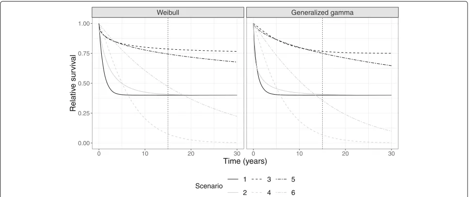
Danish general population mortality rates published by the Human Mortality Database [19]. The relative survival, R(t), was determined by a Weibull mixture cure model according to the scenarios in Fig.1. In scenario 1, 2, and 3, the cure proportion was 40%, 40%, and 75% and cure occurred within the available follow-up, just outside the follow-up, and many years after the last follow-up time, respectively. In scenarios 4, 5, and 6, the cure proportion was zero and therefore the relative survival function cor-responded to a regular Weibull model. Scenario 5 was similar to 3 within the follow-up, but differed beyond the follow-up. In scenario 4, most patients died within the follow-up and scenario 6 was included as an example of a clear absence of cure within the follow-up. In scenar-ios where R(t) had a cure proportion, follow-up times were set to∞, if there was no solution to the equation R(t) = U, whereU is uniformly distributed between 0 and 1. To examine the extrapolation performances under different trajectories, we repeated the simulations after replacing the Weibull distribution with the generalized gamma distribution.
To mimic typical register data, the censoring times were simulated from a uniform distribution,C, between 0 and 15 years. Using S∗ and R, the true loss of life-time function was obtained by inserting into (9). All scenarios were simulated 500 times with a sample size of 1000.
For estimation of the loss of lifetime function, we con-sidered five models (Table 1). In order to obtain the same number of parameters in each model, an addi-tional knot was required for model B and C, which was
placed late in the follow-up, while for model D and E the number of knots was decreased by one since these contain an explicit parameter for the cure proportion. Extrapolation using model A and B was considered by Andersson et al. [1]. We considered a special case of the latter model, where the last knot was placed beyond the available follow-up. We also considered two instances of the FMC model, i.e., D with conventional knot placement and E where the knots were placed in the beginning of the follow-up.
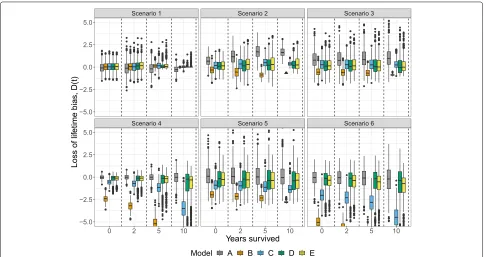
For each model, the loss of lifetime function was com-puted and the bias was measured byD(t) =L(t)−L(t). The integral,015|D(u)|du, was used to measure the bias of the loss of lifetime estimate during the entire follow-up period.
Simulation results
In scenarios with statistical cure (scenario 1, 2 and 3), all models had comparable performances at time zero for 50-year-old patients (Fig.2). In scenarios 1 and 3, the bias was fairly low for all models at all time points, but in scenario 2, the non-cure model, A, yielded increasingly upward biased estimates. In scenarios without statistical cure (scenario 4, 5, and 6), the diversity between the mod-els became larger. In these scenarios, the non-mixture cure models, B and C, underestimated the loss of life-time, most markedly seen in model B which assumes cure within the follow-up period.
Generally, the FMC models, D and E, showed good performance both in scenarios with statistical cure occur-ring within and beyond the available follow-up. In
Weibull Generalized gamma
0 10 20 30 0 10 20 30
0.00 0.25 0.50 0.75 1.00
Time (years)
Relativ
e sur
viv
al
Scenario 1
2 3
4 5
6
Table 1Specification of models used to estimate the loss of lifetime function
Model Model Nr. knots Knot locations
A NRS 6 0%, 20%, 40%, 60%, 80%, and 100%
quantiles of the uncensored event times.
B ARS 7 0%, 20%, 40%, 60%, 80%, and 100%
quantiles of the uncensored event times with an additional knot placed at 10 years.
C ARS 7 0%, 20%, 40%, 60%, and 80%
quantiles of the uncensored event times. The last knot is placed at 80 years and an additional knot is placed at 10 years.
D FMC 5 0%, 25%, 50%, 75%, and 100%
quantiles of the uncensored event times.
E FMC 5 First uncensored event time, 0.5, 1, 2, and 5 years.
NRS: Nelson et al. [10] relative survival model, ARS: Andersson et al. [13] relative survival model, FMC: Flexible mixture cure model
scenarios where statistical cure did not occur, the perfor-mance of the FMC models was comparable to model A, but the biases were more dispersed for later time point, especially in scenario 4 and 6. At ten years, the biases of model E were slightly less dispersed compared to model D.
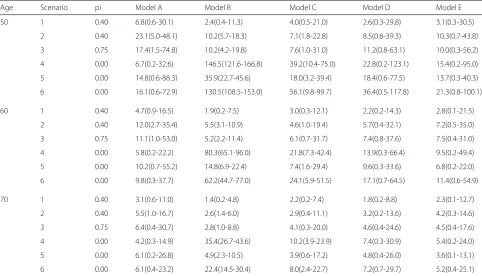
Table2shows the integrated loss of lifetime biases for 50-, 60-, and 70-year-old patients. In general, the inte-grated overall biases were consistent with Fig. 2 where model A, D, and E performed well across the six scenarios. In comparison to model D, model E was largely producing less biased estimates, while only being slightly worse than model A in scenario 4 and 6. Generally, the loss of lifetime bias decreased with increasing age and hence reduced the differences between the models. Despite the bias reduc-tion in 70-year-olds, model B still resulted in a relatively large bias in scenario 4 and 6. The results were similar in the generalized gamma case (Fig. 3 and Table 3). In particular, the models A and E showed satisfactory perfor-mance in all scenarios while model D was more biased in scenario 6. Also in the generalized gamma case, model E had slightly lower integrated bias compared to model D in scenario 4, 5, and 6.
Analysis of Danish cancer registry data
Data description
To investigate the performance of the models in Table1 in cancer survival data, we analyzed data from the Dan-ish Cancer Registry [20] on patients with colon cancer (n = 4558), breast cancer (n = 21, 731), bladder can-cer (n = 11, 738) and malignant melanoma (n = 2404). To achieve (almost) complete follow-up, we included patients diagnosed in the period 1960–1975, who were
Table 2The integrated loss of lifetime bias in the Weibull scenario, computed by integrating|D(t)|from 0 to 15 years
Age Scenario pi Model A Model B Model C Model D Model E
50 1 0.40 8.6(0.9-39.2) 2.4(0.5-10.7) 4.1(0.9-19.5) 2.4(0.2-18.5) 2.6(0.3-28.6)
2 0.40 28.9(5.5-66.9) 11.7(6.0-23.1) 12.7(3.7-35.3) 11.1(0.6-68.0) 9.3(0.7-52.1)
3 0.75 8.9(0.7-42.7) 8.9(4.3-15.6) 4.8(0.9-16.4) 7.5(0.5-31.5) 7.2(0.2-23.9)
4 0.00 6.5(0.3-34.5) 144.8(123.4-171.2) 37.2(8.9-82.1) 24.9(0.3-111.8) 18.1(0.2-104.6)
5 0.00 11.0(0.2-43.3) 25.4(14.8-35.4) 13.0(3.2-31.0) 12.8(0.4-33.8) 9.6(0.3-30.9)
6 0.00 18.1(0.5-65.4) 106.6(71.6-127.7) 49.2(7.9-92.4) 36.2(0.6-103.7) 23.9(0.2-89.4)
60 1 0.40 6.0(1.3-19.4) 1.9(0.4-8.0) 3.1(0.6-13.5) 2.1(0.2-14.7) 2.4(0.2-17.6)
2 0.40 14.9(2.6-45.4) 6.4(3.4-14.9) 7.7(2.0-26.2) 7.7(0.6-40.2) 6.6(0.2-42.5)
3 0.75 7.2(0.4-39.6) 4.2(1.9-10.0) 4.0(0.4-22.7) 5.4(0.3-28.2) 4.7(0.3-19.6)
4 0.00 5.7(0.3-24.1) 79.5(64.6-93.2) 21.0(6.1-44.4) 14.2(0.3-62.4) 10.2(0.1-49.8)
5 0.00 7.5(0.3-33.4) 10.7(5.1-18.1) 5.6(1.5-18.6) 7.2(0.5-26.0) 5.0(0.2-17.9)
6 0.00 10.9(0.6-37.3) 48.2(36.4-61.2) 18.5(4.1-42.5) 16.8(1.2-50.9) 11.2(0.3-45.3)
70 1 0.40 3.6(0.9-12.4) 1.5(0.2-4.8) 2.2(0.4-7.3) 1.7(0.1-8.8) 2.0(0.1-12.9)
2 0.40 6.2(1.2-20.8) 3.4(1.5-8.8) 4.0(0.9-14.2) 4.7(0.3-19.4) 4.3(0.3-19.2)
3 0.75 4.9(0.3-20.6) 2.4(0.8-7.0) 3.3(0.3-12.9) 3.6(0.2-19.0) 2.8(0.2-11.2)
4 0.00 4.3(0.3-16.1) 34.9(26.9-44.4) 9.6(3.5-23.3) 7.3(0.2-31.3) 5.7(0.1-27.5)
5 0.00 5.3(0.4-25.2) 3.9(1.7-8.9) 3.5(0.6-14.8) 4.3(0.2-18.5) 2.9(0.1-10.5)
6 0.00 6.0(0.3-21.7) 16.5(9.9-23.8) 6.2(1.8-16.6) 6.9(0.2-23.7) 5.1(0.2-17.4)
The loss of lifetime was computed for 50-, 60-, and 70-year-old patients. The mean and range from the 500 simulations are provided
Table 3The integrated loss of lifetime bias in the generalized gamma scenario, computed by integrating|D(t)|from 0 to 15 years
Age Scenario pi Model A Model B Model C Model D Model E
50 1 0.40 6.8(0.6-30.1) 2.4(0.4-11.3) 4.0(0.5-21.0) 2.6(0.3-29.8) 3.1(0.3-30.5)
2 0.40 23.1(5.0-48.1) 10.2(5.7-18.3) 7.1(1.8-22.8) 8.5(0.6-39.3) 10.3(0.7-43.8)
3 0.75 17.4(1.5-74.8) 10.2(4.2-19.8) 7.6(1.0-31.0) 11.2(0.8-63.1) 10.0(0.3-56.2)
4 0.00 6.7(0.2-32.6) 146.5(121.6-166.8) 39.2(10.4-75.0) 22.8(0.2-123.1) 15.4(0.2-95.0)
5 0.00 14.8(0.6-88.3) 35.9(22.7-45.6) 18.0(3.2-39.4) 18.4(0.6-77.5) 13.7(0.3-40.3)
6 0.00 16.1(0.6-72.9) 130.5(108.5-153.0) 56.1(9.8-99.7) 36.4(0.5-117.8) 21.3(0.8-100.1)
60 1 0.40 4.7(0.9-16.5) 1.9(0.2-7.5) 3.0(0.3-12.1) 2.2(0.2-14.3) 2.8(0.1-21.5)
2 0.40 12.0(2.7-35.4) 5.5(3.1-10.9) 4.6(1.0-19.4) 5.7(0.4-32.1) 7.2(0.5-35.0)
3 0.75 11.1(1.0-53.0) 5.2(2.2-11.4) 6.1(0.7-31.7) 7.4(0.8-37.6) 7.5(0.4-31.0)
4 0.00 5.8(0.2-22.2) 80.3(65.1-96.0) 21.8(7.3-42.4) 13.9(0.3-66.4) 9.5(0.2-49.4)
5 0.00 10.2(0.7-55.2) 14.8(6.9-22.4) 7.4(1.6-29.4) 9.6(0.3-33.6) 6.8(0.2-22.0)
6 0.00 9.8(0.3-37.7) 62.2(44.7-77.0) 24.1(5.9-51.5) 17.1(0.7-64.5) 11.4(0.6-54.9)
70 1 0.40 3.1(0.6-11.0) 1.4(0.2-4.8) 2.2(0.2-7.4) 1.8(0.2-8.8) 2.3(0.1-12.7)
2 0.40 5.5(1.0-16.7) 2.6(1.4-6.0) 2.9(0.4-11.1) 3.2(0.2-13.6) 4.2(0.3-14.6)
3 0.75 6.4(0.4-30.7) 2.8(1.0-8.8) 4.1(0.3-20.0) 4.6(0.4-24.6) 4.5(0.4-17.6)
4 0.00 4.2(0.3-14.9) 35.4(26.7-43.6) 10.2(3.9-23.9) 7.4(0.3-30.9) 5.4(0.2-24.0)
5 0.00 6.1(0.2-26.8) 4.9(2.3-10.5) 3.9(0.6-17.2) 4.8(0.4-26.0) 3.6(0.1-13.1)
6 0.00 6.1(0.4-23.2) 22.4(14.5-30.4) 8.0(2.4-22.7) 7.2(0.7-29.7) 5.2(0.4-25.1)
The loss of lifetime was simulated for 50-, 60-, and 70-year-old patients. The mean and range from the 500 simulations are provided
older than 50 years at diagnosis. The diseases were chosen based on the same considerations as in Andersson et al. [1], i.e., colon cancer typically displays statistical cure, bladder cancer a constant excess hazard, melanoma a rather high survival rate, and breast cancer is seen in both young and old patients. Patients were followed until the end of 2016, where alive patients were censored and follow-up was measured from diagnosis until death or censoring. For the purpose of investigating the extrap-olation performance, we restricted the follow-up to 16 years by censoring patients alive in January 1976 and divided patients into age groups; 50–59, 60–69, 70–79, 80+. The true loss of lifetime was calculated by insert-ing the Kaplan-Meier estimate into (9), and the bias was computed byD(t). For both the true and estimated loss of lifetime, the upper limit of the integrals in (9) was set to 40 years at which time the true survival was close to zero.
Results
Figure4shows the bias function for each disease and each age group using the five models in Table 1. The corre-sponding survival curves can be found in Additional file1: Figure S1-S4. The models displayed varying performance across the cancer types and age groups, but biases were commonly decreasing with increasing age. The extrapola-tion performance within bladder cancer was rather poor;
in the age groups 50–59 and 60–69, the models consis-tently underestimated the loss of lifetime function with model B being the worst. Also for breast cancer, model B underestimated the loss of lifetime function while model C, which assumes statistical cure beyond the follow-up, provided improved results. In breast cancer, the two FMC models resulted in rather different loss of lifetime biases, but the bias was not consistently better in one model. For colon cancer where statistical cure is typically dis-played, all models performed fairly well in all age groups and among the melanoma patients, model B had the best performance.
Overall, no model was consistently superior to the others, but in scenarios of statistical cure, there was a slight advantage of using cure models. However, in scenarios without statistical cure, models B and C were substantially biased.
Analysis of Danish lymphoma registry data
Data description
Bladder cancer Breast cancer Colon cancer Melanoma
50−59
60−69
70−79
80+
0 5 10 15 0 5 10 15 0 5 10 15 0 5 10 15
−3 −2 −1 0 1 2
−3 −2 −1 0 1 2
−3 −2 −1 0 1 2
−3 −2 −1 0 1 2
Years survived
Loss of lif
etime bias
, D(t)
Model A B C D E
Fig. 4Time-varying loss of lifetime bias using the models in Table1for extrapolation in bladder cancer, breast cancer, colon cancer, and melanoma patients registered in the Danish Cancer registry
n = 980) in the period from 2000 to 2016. The follow-up period was terminated in June 2017 and the follow-follow-up time was measured from time of diagnostic biopsy to death or censoring.
Population-based loss of lifetime
For each disease, three models were fitted, namely the NRS model with 6 knots, the ARS model with 7 knots, and the FMC model with 5 knots (corresponding to model A, B, and D in Table1), resulting in the same number of parameters. Additional file1: Figure S5 displays the rela-tive survival of each disease and disease-specific summary measures are shown in Table4.
The estimated loss of lifetime function based on the three models is shown for each disease in Fig.5. DLBCL
and ML patients had a high loss of lifetime at diag-nosis with a rapid decrease, while FL patients dis-played a fairly low initial loss of lifetime with a slow improvement.
Table 4Median age, 5-year relative survival (RS), and loss of lifetime estimates at time zero in Danish diffuse large B-cell lymphoma (DLBCL), follicular lymphoma (FL), and mantle cell lymphoma (ML) patients
Model DLBCL FL ML
Median age (range)
68(18-101) 63(18-97) 70(28-99)
5-year RS (95% CI)
NRS 0.66(0.65-0.68) 0.9(0.88-0.91) 0.61(0.57-0.65)
ARS 0.66(0.65-0.67) 0.9(0.88-0.91) 0.61(0.57-0.65)
FMC 0.66(0.64-0.67) 0.9(0.88-0.91) 0.61(0.58-0.65)
Loss of lifetime (95% CI)
NRS 7.43(7.06-7.80) 4.58(3.73-5.42) 7.66(6.86-8.46)
ARS 6.70(6.42-6.98) 3.57(3.13-4.02) 6.92(6.26-7.59)
FMC 7.21(6.86-7.55) 3.97(3.24-4.70) 7.74(6.95-8.53)
where cure cannot usually be assumed, this model resem-bled the NRS model and even provided slightly higher loss of lifetime estimates.
Age dependent loss of lifetime
The patient age at diagnosis plays a crucial role for the individual expected residual lifetimes and thus also the loss of lifetime function. For the NRS model, a time-dependent age effect was specified, i.e.,
R(t|a)=exp(−exp(s0(x)+sa(a)s1(x))), (11) whereais the patient age at diagnosis,sa(a) is a
spline-based age effect and s1(x) is the corresponding time-effect. For the FMC model, (8), the same model was used
for Su(t|z) and for π(z) an age dependent spline-based
logistic model,
log
π
1−π
=β0+sa(a), (12)
was chosen. Since none of the diseases showed a clear statistical cure trajectory, we did not consider the ARS model here. The number and location of the knots for the baseline spline function,s0(x), remained unchanged from “Population-based loss of lifetime” section. For sa(a), 4
knots placed at the 0%, 33%, 66%, and 100% quantiles of the patient age distribution were selected and the inter-cept was removed since this is already modelled by the baseline splines and β0. Fors1(x), the number of knots was chosen to be 3 and 2 for the NRS model and the FMC model, respectively, yielding the same total number of parameters.
The loss of lifetime conditional on 0, 2, and 5 years of survival for female patients diagnosed in 2010 is shown in Fig.6for varying patient ages. In all three cancer types, the loss of lifetime decreased with increasing diagnostic age.
For DLBCL, the two models seemed to be in agree-ment across patient age. However, the agreeagree-ment between the two models for 60–70 year old FL patients was poor, likely due to the different model assumptions. For ML, the model differences were larger for younger patients, likely due to the additional extrapolation needed to compute the loss of lifetime for these patients.
Discussion
In (8) we introduced a novel model, which incorporates statistical cure by combining regular mixture cure models with spline-based survival models. This model was com-pared to the NRS model, which has a linear effect in the spline function after the last knot and the ARS model,
DLBCL FL ML
0 3 6 9 0 3 6 9 0 3 6 9
0 2 4 6 8
Follow−up time (years)
Loss of lif
etime (y
ears)
NRS ARS FMC
DLBCL FL ML
50 60 70 80 50 60 70 80 50 60 70 80
0 5 10 15
Age at diagnosis (years)
Loss of lif
etime (y
ears)
FMC NRS Time 0 2 5
Fig. 6The loss of lifetime conditional on 0, 2, and 5 years of survival for female diffuse large B-cell lymphoma (DLBCL), follicular lymphoma (FL), and mantle cell lymphoma (ML) patients diagnosed in 2010 at varying ages
which is constant after the last knot and thereby incor-porates statistical cure. The simulations demonstrated a consistently good performance of the NRS model and the FMC model. The analysis of data from the Danish Cancer Registry did not show consistently satisfactory perfor-mance of any model, but in general assuming statistical cure at the end of the follow-up can lead to substantial biases in cases where this assumption is violated, while yielding good estimates when cure is reached. The NRS model performed slightly better than the FMC model in scenarios where statistical cure did not occur. This is likely due to the lack of identifiability often seen in cure models in cases where cure is not reached within the observed follow-up period [22], which ultimately may produce inaccurate extrapolations.
The present article expanded on the study of Andersson et al. [1] by evaluating the accuracy of the entire loss of lifetime function using three extrapolation approaches. While the loss of lifetime estimates at time zero in Fig.4 seemed to be in agreement with the results reported by Andersson et al., where only 10 years of follow-up were used, the biases were not constant over time.
The general population survival probabilities for young patients are high and precise extrapolation of the relative survival is required to avoid a biased loss of lifetime func-tion for these patients. Confirming this, we observed a higher bias among young patients which should be kept in mind when reporting loss of lifetime results. With longer follow-up and higher age, the bias will decrease and in future studies it would be of interest to estimate for a fixed age distribution, the amount of follow-up needed to provide sufficiently unbiased loss of lifetime estimates.
For some cancer types, the general population survival will likely not reflect the survival of the patients had they remained disease-free. The life style of patients diagnosed
with, e.g., lung or skin cancer is likely different from the general population life style and hence the relative sur-vival will not reflect the disease-specific (net) sursur-vival. However, this does not change the usability of the general population mortality rates to provide extrapolations of the survival function.
In contrast to net survival measures which are inter-preted in the setting where the patient can only die from the disease of interest, the loss of lifetime measure pro-vides a crude measure of the cancer-related mortality. In net measures, such as relative survival, it is often seen that elderly patients have an increased mortality since deaths from other causes are not taken into account. For young patients, even a small excess mortality may have a large impact on the loss of lifetime function as the expected life-time without cancer is long. Therefore, it is often seen that young patients have a higher loss of lifetime than elderly patients.
An alternative to the unrestricted loss of lifetime, where extrapolation is avoided, can be obtained by replacing the upper limit of the integrals in (9) by a fixed time point
τ. In this setting, pseudo-values and flexible parametric survival models have previously been recommended for computing the mean survival time [23] and could also be used for estimating the loss of lifetime function. Using the three models to estimate the restricted loss of lifetime would likely yield fairly similar estimates due to the model similarities in the first part of the follow-up (Additional file1: Figure S5). However, interpretation of the restricted loss of lifetime is not straightforward and the measure does not capture the full disease burden.
Conclusion
inconsistencies between the simulation results and the full follow-up data analysis emphasize the need for sensitivity analyses.
We therefore recommend that extensive sensitivity anal-yses are performed both with respect to the assumptions of the relative survival model as well as the number and location of the knots of the splines as recommended previously [10,13].
Additional file
Additional file 1: Supplementary figures. Description of data: Figure S1-S4 displays the extrapolated overall survival for the four cancer types considered in the analysis of data from the Danish Cancer Registry. Figure S5 displays the relative survival of the three lymphoma types considered in “Population-based loss of lifetime” section. (DOCX 248 kb)
Abbreviations
ARS: Andersson et al. [13] relative survival; DLBCL: Diffuse large B-cell lymphoma; FL: Follicular lymphoma; FMC: Flexible mixture cure; ML: Mantle cell lymphoma; NRS: Nelson et al. [10] relative survival
Acknowledgements
Not applicable.
Funding
No funding was received for the study.
Availability of data and materials
Data used to generate the findings of the study were obtained from the Danish Clinical Registries (Danish Lymphoma Registry) and the Danish Cancer Registry after approval of our study plan by both registries and the Danish Data Protection Agency. The registries contain patient identifiable information and therefore sharing of these data is not allowed per the terms of the agreement with the registries. However, from the registries, access to the data is granted on a case to case basis after submission and approval of an appropriate study plan and reasonable data request. Data from the Danish Cancer Registry can be applied for athttps://sundhedsdatastyrelsen.dk/da/ forskerservice, and data from the Danish Lymphoma Registry can be applied for athttp://www.rkkp.dk/forskning. The code used for generating the results can be found athttps://github.com/LasseHjort/LossOfLifetimeEstimation.
Authors’ contributions
The idea was conceived by LHJ, MB, and TMLA. LHJ performed all analyses and wrote the first draft of the manuscript. MB, TMLA, JLB, and TCEG contributed with essential feedback and suggestions for the methodology and the data analysis. All authors read and approved the final manuscript.
Ethics approval and consent to participate
The study was approved by the Danish Data Protection Agency
(2008-58-0028). In Denmark, no informed consent is required in order to use data from the Danish Cancer Registry and the Danish Lymphoma Registry for research purposes.
Consent for publication
Not applicable.
Competing interests
T. M.-L. Andersson is involved in an ongoing public-private real world evidence collaboration between Karolinska Institutet and Janssen Pharmaceuticals. However, the current project is not related to this collaboration.
Publisher’s Note
Springer Nature remains neutral with regard to jurisdictional claims in published maps and institutional affiliations.
Author details
1Department of Clinical Medicine, Aalborg University, Sdr. Skovvej 15, 9000
Aalborg, Denmark.2Department of Hematology, Aalborg University Hospital,
Sdr. Skovvej 15, 9000 Aalborg, Denmark.3Department of Medical
Epidemiology and Biostatistics, Karolinska Institutet, Nobels Väg, 171 65 Stockholm, Sweden.
Received: 17 November 2017 Accepted: 8 January 2019
References
1. Andersson TM-L, Dickman PW, Eloranta S, Lambe M, Lambert PC. Estimating the loss in expectation of life due to cancer using flexible parametric survival models. Stat Med. 2013;32(30):5286–300.
2. Andersson TM-L, Dickman PW, Eloranta S, Sjövall A, Lambe M, Lambert PC. The loss in expectation of life after colon cancer: a population-based study. BMC Cancer. 2015;15(1):412.
3. Bower H, Andersson TM-L, Björkholm M, Dickman PW, Lambert PC, Derolf ÅR. Continued improvement in survival of acute myeloid leukemia patients: an application of the loss in expectation of life. Blood Cancer J. 2016;6(2):390.
4. Davies C, Briggs A, Lorgelly P, Garellick G, Malchau H. The “Hazards” of Extrapolating Survival Curves. Med Dec Making. 2013;33(3):369–80. 5. Jackson C, Stevens J, Ren S, Latimer N, Bojke L, Manca A, Sharples L.
Extrapolating Survival from Randomized Trials Using External Data: A Review of Methods. Med Decis Making. 2017;37(4):377–90. 6. Hakama M, Hakulinen T. Estimating the expectation of life in cancer
survival studies with incomplete follow-up information. J Chronic Dis. 1977;30(9):585–97.
7. Lambert PC, Thompson JR, Weston CL, Dickman PW. Estimating and modeling the cure fraction in population-based cancer survival analysis. Biostatistics. 2007;8(3):576–94.
8. Royston P, Parmar MKB. Flexible parametric proportional-hazards and proportional-odds models for censored survival data, with application to prognostic modelling and estimation of treatment effects. Stat Med. 2002;21(15):2175–97.
9. Dickman PW, Sloggett A, Hills M, Hakulinen T. Regression models for relative survival. Stat Med. 2004;23(1):51–64.
10. Nelson CP, Lambert PC, Squire IB, Jones DR. Flexible parametric models for relative survival, with application in coronary heart disease. Stat Med. 2007;26(30):5486–98.
11. De Angelis R, Capocaccia R, Hakulinen T, Soderman B, Verdecchia A. Mixture models for cancer survival analysis: application to
population-based data with covariates. Stat Med. 1999;18(4):441–54. 12. Lambert PC, Dickman PW, Weston CL, Thompson JR. Estimating the
cure fraction in population-based cancer studies by using finite mixture models. J R Stat Soc: Ser C: Appl Stat. 2010;59(1):35–55.
13. Andersson TM, Dickman PW, Eloranta S, Lambert PC. Estimating and modelling cure in population-based cancer studies within the framework of flexible parametric survival models. BMC Med Res Methodol. 2011;11(1):96.
14. Ederer F, Axtell LM, Cutler SJ. The relative survival rate: a statistical methodology. Natl Cancer Inst Monogr. 1961;6:101–21.
15. Liu X-R, Pawitan Y, Clements M. Parametric and penalized generalized survival models. Stat Methods Med Res. 2018;27(5):1531–46. 16. Rutherford MJ, Crowther MJ, Lambert PC. The use of restricted cubic
splines to approximate complex hazard functions in the analysis of time-to-event data: a simulation study. J Stat Comput Simul. 2015;85(4): 777–93.
17. Clements M, Liu X-R. Rstpm2: Generalized Survival Models. 2016. R package version 1.3.4.https://CRAN.R-project.org/package=rstpm2. Accessed 1 Nov 2018.
18. Rutherford MJ, Dickman PW, Lambert PC. Comparison of methods for calculating relative survival in population-based studies. Cancer Epidemiol. 2012;36(1):16–21.
19. Human Mortality Database. University of California, Berkeley (USA), and Max Planck Institute for Demographic Research (Germany).www. mortality.org. Accessed 5 Sep 2017.
21. Arboe B, El-Galaly TC, Clausen MR, Munksgaard PS, Stoltenberg D, Nygaard MK, Klausen TW, Christensen JH, Gørløv JS, Brown PdN. The Danish National Lymphoma Registry: Coverage and Data Quality. PloS ONE. 2016;11(6):0157999.
22. Li C, Taylor J, Sy J. Identifiability of cure models. Stat Probab Lett. 2001;54(4):389–95.