Improved frequency resolution for characterization of complex fractionated atrial electrograms

R E S E A R C H

Open Access

Improved frequency resolution for

characterization of complex fractionated atrial

electrograms

Edward J Ciaccio

, Angelo B Biviano

, William Whang

and Hasan Garan

* Correspondence: [email protected]

1_{Department of Medicine, Division} of Cardiology, Columbia University Medical Center, New York, NY, USA 2

Columbia University, Harkness Pavilion 936, 180 Fort Washington Avenue, New York, NY 10032, USA

Abstract

Background:The dominant frequency of the Fourier power spectrum is useful to analyze complex fractionated atrial electrograms (CFAE), but spectral resolution is limited and uniform from DC to the Nyquist frequency. Herein the spectral resolution of a recently described and relatively new spectral estimation technique is compared to the Fourier radix-2 implementation.

Methods:In 10 paroxysmal and 10 persistent atrial fibrillation patients, 216 CFAE were acquired from the pulmonary vein ostia and left atrial free wall (977 Hz sampling rate, 8192 sample points, 8.4 s duration). With these parameter values, in the physiologic range of 3–10 Hz, two frequency components can theoretically be resolved at 0.24 Hz using Fourier analysis and at 0.10 Hz on average using the new technique. For testing, two closely-spaced periodic components were synthesized from two different CFAE recordings, and combined with two other CFAE recordings magnified 2×, that served as interference signals. The ability to resolve synthesized frequency components in the range 3–4 Hz, 4–5 Hz,. . ., 9–10 Hz was determined for 15 trials each (105 total).

Results:With the added interference, frequency resolution averaged 0.29 ± 0.22 Hz for Fourier versus 0.16 ± 0.10 Hz for the new method (p< 0.001). The misalignment error of spectral peaks versus actual values was ±0.023 Hz for Fourier and ±0.009 Hz for the new method (p< 0.001). One or both synthesized peaks were lost in the noise floor 13/105 times using Fourier versus 4/105 times using the new method. Conclusions:Within the physiologically relevant frequency range for characterization of CFAE, the new method has approximately twice the spectral resolution of Fourier analysis, there is less error in estimating frequencies, and peaks appear more readily above the noise floor. Theoretically, when interference is not present, to resolve frequency components separated by 0.10 Hz using Fourier analysis would require an 18.2 s sequence duration, versus 8.4 s with the new method.

Keywords:Atrial fibrillation, Ensemble averaging, Fourier analysis, Spectral estimation, Spectral resolution

Introduction

Accurate spectral resolution is important for analysis of atrial fibrillation (AF) in the fre-quency domain [1]. The information can be used, for example, to monitor periods of AF versus sinus rhythm in patients with paroxysmal arrhythmia. For understanding the

mechanism by which the arrhythmia is maintained, it is also desirable to quantify any temporal variation in frequency that can occur during AF [2]. Since frequency shifts can be minute, sufficient resolving power is essential to detect these differences over short time intervals. Yet this becomes more difficult when signal-to-noise ratio is low, as is often the case. Another impediment to the generation of an accurate spectral profile is the pres-ence of transients in the signal that are unrelated to physiologically relevant phenomena. One way to improve continuity in the frequency domain representation of AF from one instance of time to the next is to model and update the spectral profile based on new sig-nal information as it is acquired in atrial fibrillation sigsig-nals [2,3]. By using Gaussian func-tions to model the spectral peaks, after leveling the spectral baseline, spurious or transient changes to the signal frequency content can be excluded from the updates. When AF organization is reduced, the harmonic pattern is also expected to diminish [2], while inde-pendent spectral peaks caused for example by wavebreak can increase [4]. When resolving power is insufficient, a broad spectral peak in the Fourier power spectrum may thus be in-dicative of either a temporal variation in the frequency of a single component, or the mer-ging of multi-component independent sources [5]. Therefore, the need for sufficient spectral resolution is essential for AF analysis. Improved resolution could also be useful to study the evolution and spontaneous termination of paroxysmal AF, as well as to estimate the organization of atrial activity [6].

In recent work we introduced a paradigm for spectral estimation and signal transform-ation of complex fractionated atrial electrograms (CFAE) based upon ensemble averaging [7-9]. This relatively new technique, like Fourier analysis, depends upon the autocorrel-ation function for generautocorrel-ation of a power spectrum [9]. For spectral estimautocorrel-ation, Fourier analysis models the sinusoidal properties of the autocorrelation function, while the new technique averages the autocorrelation function at lags w, 2w, 3w, . . ., where w is the period [9]. The spectral resolution of Fourier analysis is constant across bandwidth, while the spectral resolution of the ensemble average method depends inversely on w. The 1/w relationship results in greater spectral resolution at lower frequencies, which includes the electrophysiologic range of interest of ~ 3–10 Hz that is used for AF characterization. Herein, the new technique is compared to Fourier analysis for discerning closely-spaced frequency components in CFAE, which are of interest to characterize the arrhythmia and to identify dominant frequencies.

Method

Clinical data acquisition

catheter mapping and ablation procedure. The surface electro gram signals were acquired in analog form using the GE CardioLab system (GE Healthcare, Waukesha, WI) and fil-tered from 30-500 Hz with a single-pole band pass filter to remove baseline drift and high frequency noise. The filtered signals were digitally sampled by the system at 0.977 KHz and stored. Although the band pass high end was slightly above the Nyquist frequency, negli-gible signal energy is expected to reside in this frequency range [8].

Only signals identified as CFAEs by two cardiac electro physiologists were included in the retrospective analysis. Candidate CFAE recordings of at least 10 seconds in duration were obtained from two sites outside the ostia of each of the four pulmonary veins (PV). Similar recordings were obtained at two sites on the endocardial surface of the left atrial free wall, one in the mid-posterior wall, and another on the anterior ridge at the base of the left atrial appendage. From each of these recordings, 8.4-second sequences (8192 sample points) were analyzed. A total of 240 such sequences were acquired during electrophysiolo-gic analysis–120 from paroxysmal and 120 from longstanding AF patients. Subsequently, only 216 of the recordings were determined to be CFAE, and only these were used for sub-sequent analysis. As in previous studies, all CFAE signals were normalized to mean zero and unity variance prior to further processing [9].

Frequency resolution

Using the radix-2 implementation for Fourier spectral estimation, the frequency reso-lution is:

RF ¼sample rate=discrete sample points

¼1=time duration ð1Þ

This resolution is uniform throughout the frequency range. Based upon the Nyquist the-orem, the range extends from DC to a maximum of ½ the sample rate. Atrial fibrillation signals are typically acquired at 977 Hz digitization, as was done in this study. For evalu-ation of the frequency content of CFAE, time durevalu-ations of approximately 8 seconds are de-sirable for analysis [10]. Using these parameter values, the resolution would be:

RF¼ ð977 samples=sÞ=8192 samples¼0:12 Hz ð2Þ

This frequency resolution is uniform throughout the range of DC to 977/2 = 489 Hz. The total number of data points in the resulting power spectrum will be 8192/2 = 4096. Thus the frequency resolution above the electrophysiologic range of interest, 10 Hz, to the high limit of 489 Hz, is the same as the frequency resolution within the physiologic range of 3–10 Hz.

A recently described technique that utilizes signal averaging was also used for spec-tral estimation [7-9]. Briefly, an ensemble average vector ew with dimension w × 1 is

obtained by averaging the n successive mean zero segments of a signal x having dimen-sion N × 1, with each segment being of length w:

e_w¼1=nUwx ð3aÞ

Where an underline denotes a vector, bold font indicates a matrix, Uwis the summing

matrix with dimension w × N, and Iware w × w identity submatrices used to extract the

signal segments from x. The number of signal segments in the summation is:

n¼int Nð =wÞ ð4Þ

where int is the integer function. If N/w is not an integer, then in forming Uw, 0’s are

added to the N–(nw) columns at the matrices’right edge [9]. The segment length w can be converted to a frequency:

f ¼sample rate=w ð5Þ

The power in the ensemble average is given by:

Pw¼1=w ewTew ð6Þ

To construct the power spectrum, the root mean square (RMS) power can be used [7-9]:

PwRMS¼ ffiffiffiffiffiffiffiffiffiffi

Pw

ð Þ

p

ð7Þ

which has units of millivolts. The power spectrum can be displayed by plotting

√nPwRMSversus frequency f. The √n term levels the spectral baseline, which would

otherwise decrease by 1/√n, the noise falloff per number of summations n used for en-semble averaging. Computer code to calculate this spectrum has been presented and described elsewhere [9].

From Eq. 5, it is apparent that the frequency resolution of the new spectral estimation technique is proportional to 1/w. This resolution can be calculated as:

RN¼½SR=w ½SR=ðwþ1Þ ¼fwfwþ1 ð8Þ

where RNis the resolution of the spectral estimator, SR is the sample rate, and fwand

fw+1are any two adjacent points on its frequency spectrum. The frequency resolution

will be higher (i.e., the difference fw−fw+1will be smaller) at points along the spectrum

where period w is longer (i.e. at low frequencies).

technique can be estimated from the resolution at representative frequency values. For example the resolution at 3.5 Hz is given by:

RN;3:5Hz¼977=w977=ðwþ1Þ

¼977=279977=280¼3:502 Hz3:489 Hz¼0:013 Hz ð9Þ

Similarly, the resolution at 4.5 Hz is:

RN;4:5Hz¼977=w977=ðwþ1Þ

¼977=217977=218¼4:502 Hz4:481 Hz¼0:021 Hz ð10Þ

The average resolution as determined from the resolution at 3.5, 4.5, 5.5,. . ., 9.5 Hz is 0.05 Hz. However to resolve two peaks, there must be at least one point of power spectral resolution separating them. Thus the minimum frequency at which two spectral peaks can be resolved would be 2 × 0.12 Hz = 0.24 Hz for Fourier, and on the average 2 × 0.05 Hz = 0.10 Hz for the new method in the range 3–10 Hz (see second column, Table 1). As a note of comparison, to theoretically resolve frequency components separated by 0.10 Hz using Fourier analysis would therefore require an 18.2 s sequence duration, ver-sus 8.4 s with the new method.

Synthesis of simulated CFAE and power spectra

CFAE with closely-spaced frequency components were artificially synthesized to test the resolution of the methods as follows. First a sequence of random length ωwas extracted from one of the 216 CFAE recordings, which was also selected at random. The extracted sequence of lengthωwas repeated to N = 8192 sample points to form one signal compo-nent. Then another random sequence, with lengthω+ 2, was extracted from another ran-domly selected CFAE recording. The extracted sequence of lengthω+ 2 was also repeated to N = 8192 sample points to form a second signal component. Two other of the 216 CFAE recordings selected at random were each amplified with a gain of ×2 to be used as interference as in a previous study [8]. Thus the following four randomly obtained sequences of length 8192 sample points were summed and used for subsequent analysis:

1. signal component 1 with repeating period w 2. signal component 2 with repeating period w + 2 3. interference 1 with 2× gain

4. interference 2 with 2× gain

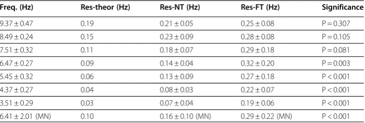
Table 1 Resolution to discern closely-spaced frequency components

Freq. (Hz) Res-theor (Hz) Res-NT (Hz) Res-FT (Hz) Significance

9.37 ± 0.47 0.19 0.21 ± 0.05 0.25 ± 0.08 P = 0.307

8.49 ± 0.24 0.15 0.23 ± 0.09 0.28 ± 0.08 P = 0.105

7.51 ± 0.32 0.11 0.18 ± 0.07 0.29 ± 0.18 P = 0.081

6.47 ± 0.27 0.09 0.14 ± 0.04 0.32 ± 0.20 P = 0.003

5.45 ± 0.32 0.06 0.13 ± 0.09 0.27 ± 0.18 P < 0.001

4.37 ± 0.27 0.04 0.08 ± 0.03 0.22 ± 0.07 P < 0.001

3.51 ± 0.29 0.03 0.07 ± 0.04 0.19 ± 0.06 P < 0.001

6.41 ± 2.01 (MN) 0.10 0.16 ± 0.10 (MN) 0.29 ± 0.22 (MN) P < 0.001

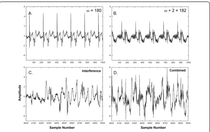
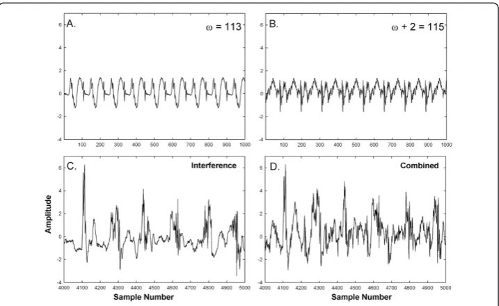
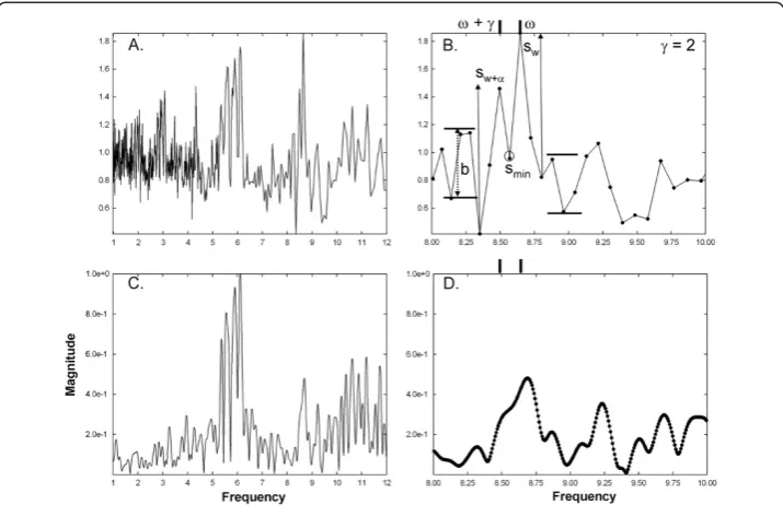
An example of the synthesis process is shown in Figure 1 for frequencies toward the low end of the spectral range. Repeating segments withω= 180 sample points andω+ 2 = 182 sample points are shown in panels A and B, respectively (f = 5.43 Hz and 5.37 Hz). The sum of two additive interferences with a gain of 2× is shown in panel C. The result from combining the components of panels A, B, and C is shown in panel D. The original peri-odicities are mostly unrecognizable in panel D. Similarly, an example for components with frequencies toward the high end of the electrophysiologic range of interest is shown in Figure 2. Repeating segments withω= 113 sample points andω+ 2 = 115 sample points are shown in panels A and B, respectively (f = 8.65 Hz and 8.50 Hz). Additive interferences are shown in panel C. The result from combining the components of panels A, B, and C is shown in panel D. The original periodicities are again mostly unrecognizable.

This paradigm was repeated so that a total of 15 simulated CFAE with closely-spaced fre-quency components in the range 3–4 Hz, 15 in the range 4–5 Hz,. . ., and 15 in the range 9–10 Hz were constructed. Thus the total number of simulation signals to be analyzed, of the type shown in Figure 1D and 2D, was 7 × 15 = 105.

Prior to Fourier analysis, each simulated signal was zero-padded to a length N = 65536, for a final interval of 0.015 Hz between spectral points. By zero padding, the frequency resolution of the FFT was not increased, only the point-to-point interval in the resulting spectrum, because the length of the observed signal was unchanged. Zero padding ensured that closely-spaced spectral components would be evident within the limit given by the fre-quency resolution constraint. The Fourier power spectrum was generated using a radix-2 implementation [11]. Initially the simulated CFAE were preprocessed with a Han window prior to Fourier analysis. However, while Han windowing can improve periodicity by for-cing the signal ends to zero, it also adds distortion in the form of amplitude modulation. The amplitude modulation can impart spectral sidebands which reduce frequency

resolution. It was also observed visually that discernment of closely-spaced frequency com-ponents was improved without this filter. Therefore a rectangular window (i.e. no filter) was used for Fourier analysis. Likewise, no window preprocessing was done prior to spec-tral estimation with the new method.

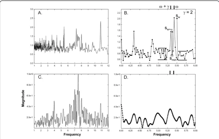
Consider the spectral profiles of both Fourier and new technique, each of which consists of 4096 data points for parameter values of 977 Hz sample rate and a signal length of 8192 sample points. As shown in Figures 1 and 2, the initially synthesized signals had frequency components of ω and ω+γ, whereγ= 2, the minimum resolving distance. To determine the ability of each method to resolve closely-spaced peaks,γwas increased by 1 in each of the simulated signals until two distinct peaks appeared in the spectrum. Closely-spaced synthesized frequency components were considered to be resolved for the minimum value ofγfor which any resulting spectral peaks with periods w and w +αmet the following four criteria. The first requirement for discernability was that:

s2>s1=4 ð11Þ

where s is the amplitude of the tallest spectral peak in proximity to the actual location of a synthesized frequency component, referenced to that foot which gives the largest peak amplitude, s1is the amplitude of the higher peak, and s2is the amplitude of the lower peak.

An example of peak amplitude measurement is shown in Figure 3B (solid vertical arrows). The second requirement for discernability is that the minimum value between the two peaks:

smin¼min s½ wþ1:swþα1 ð12Þ

is within or below the maximum range b of the neighboring background level (Figure 3B). The neighboring background level is defined as the range in magnitude −0.25 Hz in

frequency away from the left foot of peak w +α, and +0.25 Hz in frequency away from the right foot of peak w (horizontal lines, Figure 3B). The third criterion is that:

sw;swþα>b ð13Þ

that is, the magnitudes swand sw+αare greater than the maximum range b of the

neighbor-ing background level (Figure 3B). The final criterion is that the peaks at w and w +αare each within ±0.15 Hz of the two synthesized frequency components having actual periods ofωandω+γ(noted with bars at the top of the graph in Figure 3B).

The spectral resolution of Fourier analysis versus the new technique in the presence of interference were determined as follows. The criteria as given by Equations 11, 12 and 13 were tested for two synthesized spectral components with periods ω and ω+γ, γ= 2 through 20 spectral points. Again, the lower limit of 2 was necessitated by the fact that two frequency components occurring at adjacent spectral points (γ= 1) cannot be resolved. The minimum value ofγ for which these criteria were met was defined as the spectral resolution to discern the closely-spaced simulated spectral peaks. If these criteria were not met toγ= 20, the trial was tabulated as being one in which the resolution was in-determinable due to the loss of one or more spectral peaks in the noise floor. For both methods, the estimate error was defined as the average of the absolute difference in fw- fω

and fw+α –fω+γ, where fwand fω are the measured and actual frequencies of one of the

peaks, and fw+α and fω+γ are the measured and actual frequencies of the other peak,

re-spectively. For Fourier analysis, a correction was made by subtracting 0.06 Hz from each error after calculating the absolute difference of measured to actual frequency, with the

minimum error after subtraction being 0.00 Hz. This allowed for the fact that for simpli-city, the synthetic frequencies that were used were always 1/w, with w being an integer, so that on average for Fourier analysis, having constant increments of 0.12 Hz between spec-tral points, the actual frequency components could be different by as much as ±0.06 Hz. For the new technique, the spectral points occurred at 1/w for all w in range, so no cor-rection was done.

The overall paradigm was repeated for 15 trials in each frequency range 3–4 Hz, 4–5 Hz, . . ., 9–10 Hz for both Fourier analysis and the new technique. The results were averaged and tabulated as mean ± standard deviation. The unpairedt-test was used to determine the significance of the difference between methods (SigmaPlot 2004 for Windows Ver. 9.01, Systat Software, Chicago, and MedCalc ver. 9.5, 2008, MedCalc Software bvba, Mariakerke, Belgium).

Results

Spectral properties

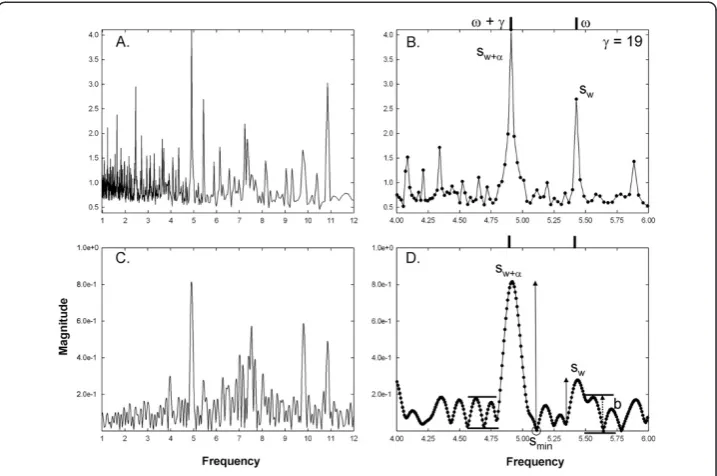
A power spectrum using the new spectral estimation technique is shown in Figure 3A. Note that the highest frequency resolution occurs at lower frequencies due to the 1/w re-lationship of resolution to frequency for this method. By comparison, the Fourier power spectrum is uniform in resolution across the range (Figure 3C). Figures 3B and D show close-ups of the respective spectra in the range of the synthesized components. The actual synthesized components have frequencies of 5.34 Hz (ω+γ= 183 sample points at 977 Hz sampling rate) and 5.43 Hz (ω= 180 sample points), noted by vertical bars at the tops of panels 3B and 3D. The two components are correctly resolved by the new technique (panel 3B), that is, w =ω and w +/=ω+γ. However, Fourier analysis does not resolve at this component spacing (panel 3D). In Figure 4, using the same CFAE and with the high frequency remaining at 5.43 Hz (ω= 180 sample points), the result is shown forγ= 19 when the low frequency is 4.91 Hz (ω+γ= 199 sample points). The spectrum and close-up using the new method are shown in Figure 4A-B, and the frequency components are readily resolved as in Figure 3A-B. The Fourier spectrum is shown in Figure 4 C-D and now distinct peaks appear (Figure 4D), meeting the criteria set forth in the Methods. This was the minimum distanceγat which two corresponding Fourier spectral peaks met the criteria, and therefore the resolution for the Fourier spectrum. The measurements for sw+α, sw, smin, and b are shown.

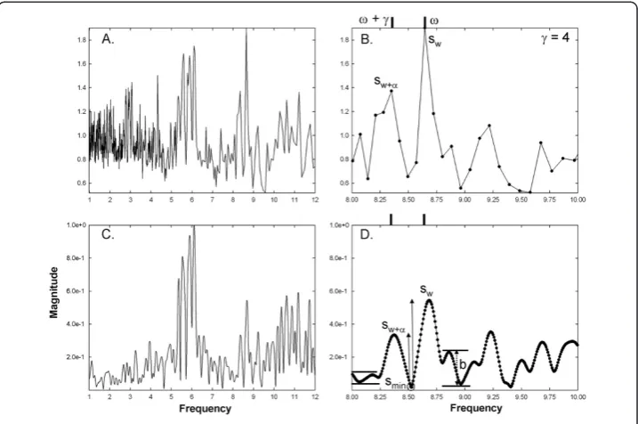
The power spectrum from 1–12 Hz using the new technique with a different set of sig-nals, and synthesized components near the higher end of the frequency range is shown in Figure 5A. The components reside at fω+γ= 8.50 Hz and fω= 8.65 Hz. Several subharmonics

Fourier analysis (Figure 6D). The actual frequency components have values of fω+γ= 8.35 Hz and fω= 8.65 Hz. The parameters indicating that the Fourier spectral peaks

resolve are noted (Figure 6D).

Summary statistics

For a total of 105 trials, excluding those in which the synthesized components could not be resolved, the mean frequency resolution with the presence of additive interference was 0.29 ± 0.22 Hz for Fourier and 0.16 ± 0.10 Hz for the new technique (p< 0.001). Thus the re-solving power of each method, in the presence of interference, was similar to their respect-ive theoretical resolutions of 0.10 Hz and 0.24 Hz. A complete summary of the resolving power of both techniques is provided in Table 1. The mean frequency for the random trials in each frequency bin that resolved are shown in the rows of column 1 from top to bottom (9–10 Hz, 8–9 Hz, . . .). The expected resolution at 9.5 Hz, 8.5 Hz, . . ., using the new method, are noted in the second column. The actual resolving power for the new technique and for the Fourier transform are shown in the next two columns, respectively. At all fre-quencies, the new technique resolving power is improved over the Fourier method. The sig-nificance of the difference in mean resolving power between the methods is noted in the right-hand column. At lower frequencies up to 7 Hz there is a highly significant difference (p≤0.003). At higher frequencies the difference trends toward significance.

The average of the absolute misalignment of spectral peaks with actual values of synthesized components (the estimate error) was 0.023 ± 0.039 Hz for Fourier and 0.009 ± 0.030 Hz for the new technique (p< 0.001). A complete summary of the esti-mate error for both methods is provided in Table 2. The mean frequency for the trials

in each frequency bin that resolved is again shown in the rows of column 1 from top to bottom, as in Table 1. The estimate error values for each frequency bin are shown for the new technique and for Fourier analysis in the middle columns. In each case, the error, or misalignment of spectral peak with respect to actual component frequencies, is substantially less using the new technique. The significance of the difference in error between the new technique and Fourier analysis is noted in the right-hand column. There is a high degree of significance at all frequencies except the 9–10 Hz bin.

Overall, of 15 trials for each frequency bin (105 trials in all), one or both frequency components did not appear above the noise floor in 13/105 trials using the Fourier method (12.4%) versus 4/105 trials using the new technique (3.8%).

Discussion Summary

In this study a comparison was made between the ability to resolve two closely-spaced fre-quency components in the physiologic range of interest using Fourier power spectral ana-lysis, versus a new technique that utilizes signal averaging. The synthesized closely-spaced frequency components and two additive interferences were selected at random from a set of 216 CFAE. The values for digital sampling rate (977 Hz) and sequence length (N = 8192, 8.4 s sequences) are typical of those used for frequency analysis of CFAE obtained during clinical EP study. Tests were made in the range 3–10 Hz, the electrophysiologic range for evaluation of atrial electrical activity. From 105 tests, the mean resolving power of Fourier versus the new technique (0.29 Hz versus 0.16 Hz;p< 0.001), were higher than the theoret-ical values but in accord with the presence of large interferences that could act to mask the

frequency components. In 13/105 trials, interference masked frequency components in the Fourier power spectrum. By comparison, this occurred in only 4/105 trials using the new technique. The error in estimating the synthesized components was ±0.023 Hz using Fou-rier versus ±0.009 Hz using the new technique (p< 0.001).

Signal segment not used for spectral estimation

Based upon Eq. 4, whenever n is not an integer, a portion of the 8.4 second CFAE sig-nal at its end is not used for spectral estimation. This can be described as:

L¼½N=wint Nð =wÞ=977 ð14Þ

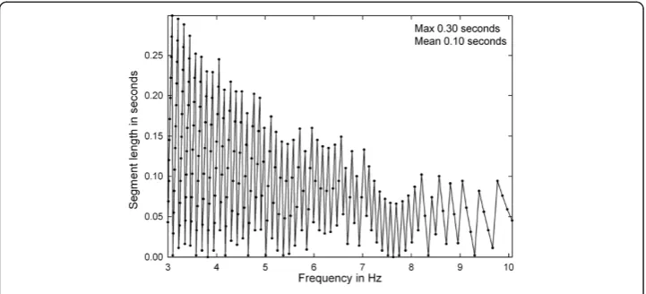
where L is the unused signal segment length in seconds. In Figure 7 is shown a plot of segment length versus frequency in the physiologic range of interest (3–10 Hz). The

Table 2 Estimate error in the frequency of peak values

Freq. (Hz) Error NT (Hz) Error FT (Hz) Significance

9.37 ± 0.47 0.032 ± 0.074 0.039 ± 0.070 P = 0.708

8.49 ± 0.24 0.004 ± 0.003 0.016 ± 0.015 P < 0.001

7.51 ± 0.32 0.004 ± 0.002 0.027 ± 0.043 P = 0.006

6.47 ± 0.27 0.005 ± 0.007 0.017 ± 0.023 P = 0.011

5.45 ± 0.32 0.003 ± 0.002 0.018 ± 0.023 P = 0.001

4.37 ± 0.27 0.003 ± 0.002 0.019 ± 0.019 P < 0.001

3.51 ± 0.29 0.013 ± 0.035 0.043 ± 0.053 P = 0.016

6.41 ± 2.01 (MN) 0.009 ± 0.030 (MN) 0.023 ± 0.039 (MN) P < 0.001

Freq.: the mean frequency used for the test, Error–NT: the difference between the actual and estimated frequency using the new method, Error–FT: the absolute difference between actual and estimated frequency using Fourier analysis, Significance–the significance of the difference between the techniques based on the unpairedt-test. MN–mean value.

maximum unused segment length, 0.3 seconds, occurs at 3.1 Hz, near the lowest fre-quency in the range. The mean unused segment length is approximately 0.1 seconds. Thus on the average, 8.3 seconds of the 8.4 second signal is used for power spectral es-timation, meaning that only about 1% of the signal is not included in the measurement.

Clinical correlates

The dynamics of internal fibrillatory activity are of great interest to establish AF mechanisms as well as for catheter ablation, and can be measured using markers of organization [12]. It would be desirable to correlate these invasive measurements with noninvasive electrocardiogram measurements, to determine the extent to which AF can be characterized noninvasively with for example, a Holter monitor [12]. It is also desirable to distinguish slightly different levels of organization during AF by improving temporal resolution and sensitivity [13]. Such improvements could lead to new ways of analyzing and understanding AF, and improved AF treatment methods [13]. The para-meters used in our study for analysis of CFAE are typical for clinical investigations. The capability of the Fourier transform to resolve two independent frequency components in close proximity, 0.24 Hz, is unacceptable for describing the temporal evolution of paroxysmal AF or to differentiate this type from persistent AF. Using Fourier analysis, the dominant frequency, defined as the tallest spectral peak in the physiologic range of interest, often varies with a standard deviation of 0.2–0.3 Hz when CFAE are recorded from each of the four pulmonary vein ostia [14]. Thus the resolving power using the Fourier spectrum is likely to be insufficient for detailed, accurate measurement. To de-termine whether differences in the frequencies of spectral peaks are real or artifact requires an increase in resolving power, as is possible with our new technique. Further-more, the ability to resolve multiple characteristic frequencies in AF signals, which may be caused by multiple wavelets propagation as are commonly found in AF data, is more difficult when the electrical activity is highly unorganized [15]. Applying the new tech-nique to these signals can potentially increase the ability to spectrally resolve the mul-tiple activation wavelets that can be present in the arrhythmogenic substrate.

Conclusions

In this study we demonstrated that the resolving power to discern two closely-spaced synthe-sized frequency components was significantly greater using a new spectral estimation tech-nique as compared with Fourier analysis. Furthermore, the new techtech-nique estimates the actual frequencies of the components to a significantly greater degree of accuracy as com-pared with Fourier. The simulations suggest that two closely-spaced frequency components, as might be encountered by drivers of electrical activation in close spatial proximity to one another within the arrhythmogenic substrate that is causing atrial fibrillation, can be dis-cerned by the new technique, even in combination with substantial interference levels. Such interferences may represent, for example, independent drivers at the periphery of the sub-strate that are inconsequential to the maintenance of AF. Thus this method may be helpful to detect and identify independent drivers in the atrial substrate that can be masked by inter-ference from bystander regions. Such information is potentially important to develop a mech-anistic understanding of the pattern of electrical activation during atrial fibrillation. Although only CFAE simulations were done in this study, these observations are probably applicable to other types of signals including ventricular electrograms [16] and electrocardiogram data [17]. Furthermore, better spectral resolution can be important for improved recognition of repeating patterns in CFAE when analyzed in the frequency domain [18].

Limitations

For simplicity, the number of trials for discerning closely-spaced frequency components was limited to 15 for each of seven frequency bins in the electrophysiologic range of interest. The types of interference signals and the types of periodic components that were used were limited to those present in a pool of 216 CFAE recordings obtained from the pulmonary vein ostia and left atrial free wall in both paroxysmal and longstanding AF patients. The use of synthesized components was necessitated by the fact that frequency values needed to be known with certainty. Since synthesized signals were tested, they will not necessarily repre-sent the performance of Fourier spectral analysis versus the new technique on real data. Still, since the synthesized frequency components and interferences were extracted from real CFAE, we believe that they are representative of the types of signals that would be encoun-tered in real measured data.

Competing interests

The authors declare that they have no competing interests.

Author contributions

EJC developed the mathematical methods, conducted the data analysis, and wrote the manuscript. ABB, WW, and HG made helpful suggestions, provided the clinical data, and determined which recordings were complex fractionated atrial electrograms. All authors have read and approved the final manuscript.

Acknowledgements

We would like to thank Dr. Niels F. Otani, Mohammed M. Premjee, and Dr. Laura M. Muñoz of the Department of Biomedical Sciences at Cornell University, and Dr. Elisa Konofagou, Dr. Jean Provost, and Alexandre Costet of the Department of Biomedical Engineering at Columbia University, for very helpful discussions. No outside funding was received for this study.

Received: 13 January 2012 Accepted: 13 March 2012 Published: 3 April 2012

References

2. Corino VD, Mainardi LT, Stridh M, Sörnmo L:Improved time-frequency analysis of atrial fibrillation signals using spectral modeling.IEEE Trans Biomed Eng2008,55:2723–2730.

3. Stridh M, Sornmo L, Meurling C, Olsson SB:Sequential characterization of atrial tachyarrhythmias based on ECG time-frequency analysis.IEEE Trans Biomed Eng2004,51:100–114.

4. Zlochiver S, Yamazaki M, Kalifa J, Berenfeld O:Rotor meandering contributes to irregularity in electrograms during atrial fibrillation.Hear Rhythm2008,5:846–854.

5. Huang Z, Chen Y, Pan M:Time-frequency characterization of atrial fibrillation from surface ECG based on Hilbert-Huang transform.J Med Eng Technol.2007,31:381–389.

6. Vayá C, Rieta JJ:Time and frequency series combination for non-invasive regularity analysis of atrial fibrillation.Med Biol Eng Comput2009,47:687–696.

7. Ciaccio EJ, Biviano AB, Whang W, Wit AL, Garan H, Coromilas J:New methods for estimating local electrical activation rate during atrial fibrillation.Hear Rhythm2009,6:21–32.

8. Ciaccio EJ, Biviano AB, Whang W, Wit AL, Coromilas J, Garan H:Optimized measurement of activation rate at left atrial sites with complex fractionated electrograms during atrial fibrillation.J Cardiovasc Electrophysiol 2010,21:133–143.

9. Ciaccio EJ, Biviano AB, Whang W, Coromilas J, Garan H:A new transform for the analysis of complex fractionated atrial electrograms.BioMed Eng OnLine2011,10:35.

10. Biviano AB, Coromilas J, Ciaccio EJ, Whang W, Hickey K, Garan H:Frequency domain and time complex analyses manifest low correlation and temporal variability when calculating activation rates in atrial fibrillation patients.Pacing Clin Electrophysiol2011,34:540–548.

11. Numerical Recipes in Fortran.Cambridge, UK: Cambridge University Press; 1992.

12. Alcaraz R, Hornero F, Rieta JJ:Assessment of non-invasive time and frequency atrial fibrillation organization markers with unipolar atrial electrograms.Physiol Meas2011,32:99–114.

13. Sih HJ, Zipes DP, Berbari EJ, Olgin JE:A high-temporal resolution algorithm for quantifying organization during atrial fibrillation.IEEE Trans Biomed Eng1999,46:440–450.

14. Ng J, Kadish AH, Goldberger JJ:Technical considerations for dominant frequency analysis.J Cardiovasc Electrophysiol2007,18:757–764.

15. Nguyen MP, Schilling C, Dossel O:A new approach for frequency analysis of complex fractionated atrial electrograms.Conf Proc IEEE Eng Med Biol Soc2009,2009:368–371.

16. Ciaccio EJ, Tennyson CA, Bhagat G, Lewis SK, Green PH:Robust spectral analysis of videocapsule images acquired from celiac disease patients.BioMed Eng OnLine2011,10:78.

17. Ciaccio EJ, Drzewiecki GM:Tonometric arterial pulse sensor with noise cancellation.IEEE Trans Biomed Eng2008, 55:2388–2396.

18. Ciaccio EJ, Biviano AB, Whang W, Garan H:Identification of recurring patterns in fractionated atrial electrograms using new transform coefficients.BioMed Eng OnLine2012,11:4.

doi:10.1186/1475-925X-11-17

Cite this article as:Ciaccioet al.:Improved frequency resolution for characterization of complex fractionated atrial electrograms.BioMedical Engineering OnLine201211:17.

Submit your next manuscript to BioMed Central and take full advantage of:

• Convenient online submission

• Thorough peer review

• No space constraints or color figure charges

• Immediate publication on acceptance

• Inclusion in PubMed, CAS, Scopus and Google Scholar

• Research which is freely available for redistribution