Model selection in Medical Research: A simulation study comparing Bayesian Model Averaging and Stepwise Regression

R E S E A R C H A R T I C L E

Open Access

Model selection in Medical Research: A simulation

study comparing Bayesian Model Averaging and

Stepwise Regression

Anna Genell

, Szilard Nemes

, Gunnar Steineck

, Paul W Dickman

Abstract

Background:Automatic variable selection methods are usually discouraged in medical research although we believe they might be valuable for studies where subject matter knowledge is limited. Bayesian model averaging may be useful for model selection but only limited attempts to compare it to stepwise regression have been published. We therefore performed a simulation study to compare stepwise regression with Bayesian model averaging.

Methods:We simulated data corresponding to five different data generating processes and thirty different values of the effect size (the parameter estimate divided by its standard error). Each data generating process contained twenty explanatory variables in total and had between zero and two true predictors. Three data generating processes were built of uncorrelated predictor variables while two had a mixture of correlated and uncorrelated variables. We fitted linear regression models to the simulated data. We used Bayesian model averaging and stepwise regression respectively as model selection procedures and compared the estimated selection probabilities. Results:The estimated probability of not selecting a redundant variable was between 0.99 and 1 for Bayesian model averaging while approximately 0.95 for stepwise regression when the redundant variable was not correlated with a true predictor. These probabilities did not depend on the effect size of the true predictor. In the case of correlation between a redundant variable and a true predictor, the probability of not selecting a redundant variable was 0.95 to 1 for Bayesian model averaging while for stepwise regression it was between 0.7 and 0.9, depending on the effect size of the true predictor. The probability of selecting a true predictor increased as the effect size of the true predictor increased and leveled out at between 0.9 and 1 for stepwise regression, while it leveled out at 1 for Bayesian model averaging.

Conclusions:Our simulation study showed that under the given conditions, Bayesian model averaging had a higher probability of not selecting a redundant variable than stepwise regression and had a similar probability of selecting a true predictor. Medical researchers building regression models with limited subject matter knowledge could thus benefit from using Bayesian model averaging.

Background

Automatic variable selection methods are usually dis-couraged in medical research although we believe they might be valuable for studies where subject matter knowledge is limited. Bayesian model averaging [1] may be useful for model selection; it may be worthwhile to further investigate its performance compared to

commonly used automatic selection procedures such as stepwise regression.

The context of this study is a class of observational studies where we hope to identify predictors of a single outcome from within a range of 20-40 possible explana-tory variables. We are particularly interested in the situation where we have been the first, or among the first, to collect empirical data in a research field and subject matter knowledge is therefore nonexistent or extremely limited. Our interest is not on testing a lim-ited number of well-defined hypotheses but on * Correspondence: [email protected]

1

Clinical Cancer Epidemiology, Department of Oncology, Institute of Clinical Sciences, Sahlgrenska University Hospital, Gothenburg, Sweden

Full list of author information is available at the end of the article

describing associations between potential predictors and the outcome. It is, if not impossible, hard to manually assess all combinations of predictor variables even when we ignore the possibility of interactions. In such scenar-ios there are strong arguments for making use of data-driven model selection methods (ideally in conjunction with subject matter knowledge if there is any). In this context false positives (type I error) can be a major pro-blem [2-4].

The most well-known and widely-applied such method is stepwise regression which has been shown to perform poorly in theory, case-studies, and simulation [2-6]. Also, it is generally desirable to validate each step of the model building process [7] including model selection.

Wang and coworkers compared, in a simulation study [8], Bayesian model averaging to stepwise regression. They found that Bayesian model averaging ‘chose the optimal model eight to nine out of ten simulations’. However, they did not perform more than ten simula-tions, so the possibility that their conclusions were dependent on random chance cannot be excluded. Also, Wang and coworkers did not mention any controlling or variation of the effect size of a true predictor and they did not examine the situation where a redundant variable is correlated with a true predictor. Also Raftery and coworkers performed a simulation study [2] and found that in ten simulations of a null model (no pre-dictor variables were related to the outcome variable), the built-in selection method ("Occam’s window”) in Bayesian model averaging chose the null model or mod-els with just a few variables whereas stepwise regression chose models with many variables.

The classical a -level of 0.05 is historically accepted and is a convention in the scientific community. One might intuitively use the posterior probability in BMA in a similar way and therefore use a 95% threshold although the convention in the Bayesian model aver-aging litterature is using a 50% posterior probability threshold as analogous to the frequentist 0.05 signifi-cance level [9,10].

In this study we use linear regression to examine and compare stepwise regression (using Akaike Information Criterion (AIC) for model building together with 0.05 significance criteria for inclusion in the final model) with Bayesian model averaging (applying both a 50% and a 95% posterior probability threshold) in terms of selecting true predictors and redundant variables by simulating data corresponding to five different data gen-erating processes and thirty different values of effect size of a true predictor and then analyzing the simulated data with Bayesian model averaging and stepwise regres-sion respectively. We chose to perform our study in the framework of linear regression to facilitate greater

control of the effect size of true predictors (the para-meter estimate divided by its standard error).

Methods

Data simulation

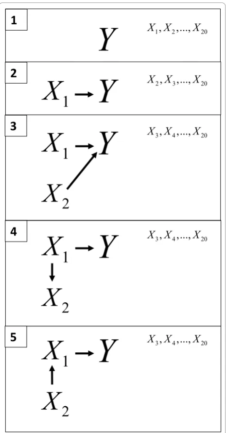
We designed 5 different data generating processes that can be said to represent a hypothetical cross-sectional study containing one outcome, Y, which was condi-tioned on 0, 1 or 2 of the 20 remaining variables X1, ...

X20.

The outcome Y_jkl was generated as follows:

Y_{jkl i}x

i ijkl jkl

=

∑

1 20

, wherei denotes twenty

differ-ent variables,jdenotes five data generating processes,

kdenotes thirty different values of the residual variance,

ldenotes 300 simulations andεjkl~ N(0,sk),s1= 0.5,...,

s30= 80 with the increment 2.74. The five data generat-ing processes, which are described graphically in Figure 1 were specified as

1.bi= 0∀i

2.b1= 1 andbi= 0∀i> 1 3.b1= 1,b2= 1 andbi= 0∀i> 2

4.b1 = 1 and bi= 0 ∀i > 1 and X2=X1jkl+X2jkl ,

where X2jkl ~N(0, 1)

5.b1 = 1 and bi = 0 ∀i > 1 and X1=X2jkl +X1jkl ,

where X1jkl ~N(0, 1)

In each of a series of 300 simulations we commenced by generating 500 observations of 20 independent, iden-tically distributed random variables from a standard nor-mal distribution. For data generating process 4, the redundant variablex2 was generated from the true pre-dictor x1, and in data generating process 5 the true pre-dictorx1 was generated fromx2. Therefore, x2 in data generating process 4 andx1 in data generating process 5 did not have standard normal distributions.

We define variables used for generating the outcome as true predictors and the remaining variables as redundant variables. We varied the effect size of the true predictor (where we define effect size as the parameter estimate divided by its standard error) by adding to the data gen-erating process an error variable with mean zero and a range of 30 different values of the variance. We regard the data generating process 1 as being less complex than data generating process 2, which in turn is less complex than data generating process 3, and so on.

because for a fixed b, the effect size of the true tor (and thus the probability of selecting a true predic-tor) is dependent on the amount of noise. The simulations were performed in R [11] using the function

rnorm (which uses the Mersenne-Twister random number generator). A random seed was generated for each simulation.

Data analysis

For each of the five data generating processes and each of the 30 values of effect size, we analyzed each of the 300 simulated data sets using both Bayesian model

averaging and forward stepwise regression selection with the Akaike Information Criterion (AIC) as the step cri-teria [12]. As a final step in stepwise regression we excluded all previously selected variables with a p-value of 0.05 or greater. We will refer to this as stepwise regression. In Bayesian model averaging we made use of the posterior probabilities given for each variable and introduced on one hand a 95% threshold and on the other hand a 50% threshold for the posterior probabil-ities for the variables in the averaged model. The 95% threshold was motivated by the approach a first time user might naively take. The 50% threshold was moti-vated by convention in the Bayesian model averaging lit-erature [9,10]. We thus defined variables having a posterior probability below 95% and 50% respectively as selected. We aimed to study a situation where subject matter knowledge is extremely limited. When analysing the data we assumed no existing subject matter knowl-edge. Therefore, for Bayesian model averaging we used noninformative priors. Further, we used Gaussian error distribution, constant equal to 20 in the first principle of Occam’s window and non-strict Occam’s window. The analyses were performed in R [11] using the lm and step functions and, for Bayesian model averaging, the bic.glm function in the BMA package [13,14]. An overview of Bayesian model averaging is given in the appendix.

Method comparison

We compared the selection methods in terms of the probability of selecting a true predictor and the prob-ability of not selecting a redundant variable. For each method, we estimated the probability of selecting a true predictor as the proportion of cases where a true predic-tor was selected and the probability of not selecting a redundant variable as the proportion of cases where a redundant variable was not selected. We also compared the probability of selecting the correct model which we estimated as the proportion of cases where the true pre-dictor or prepre-dictors (in the case of two true prepre-dictors) was selected and no other variables were selected. For the null hypothesisH0 :bi= 0, the probability of select-ing a true predictor corresponds to the probability of rejectingH0given it is false and the probability of not selecting a redundant variable corresponds to the prob-ability of failing to rejectH0 given it is true.

Results

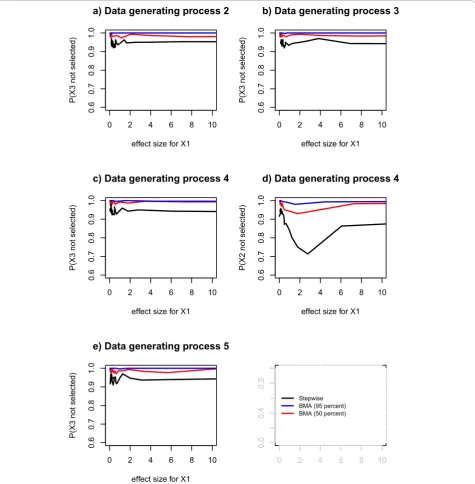
Probability of not selecting a redundant variable

For data generating process 1, Bayesian model averaging with 95% threshold almost never (less than 1 time per hundred) selects redundant variables, Bayesian model averaging with 50% threshold selects a redundant vari-able 1 time per hundred and stepwise regression selects a redundant variable with probability 0.05 (data not

Y

Y

Y

1

X

1

X

2

X

1

X

2

X

1

X

2

X

1

,

,...,

X X

X

2

,

,...,

X X

X

3

,

,...,

X X

X

3

,

,...,

X X

X

3

,

,...,

X X

X

Y

Y

1

2

4

5

3

shown). These probabilities are independent of the effect size of the true predictor. This holds for the other data generating processes when considering redundant variables that are uncorrelated with a true predictor (Figure 2a, b, c and 2e). The exception to the pattern was data generating process 4 when a redundant vari-able was correlated with a true predictor. In this case the probability of selecting a redundant variable was dependent on the effect size of the true predictor. Above an effect size corresponding to a t-test statistic of 2, the probability of not selecting a redundant variable varied between approximately 0.7 and 0.9 for stepwise regression. For Bayesian model averaging with 50% threshold it varied between approximately 0.8 and 1. For Bayesian model averaging with 95% threshold it was approximately 1(Figure 2d).

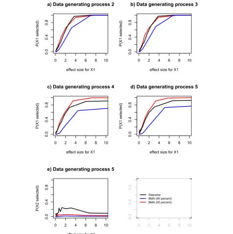
Probability of selecting a true predictor

We observed that the probability of selecting a true pre-dictor increased as the effect size of the true prepre-dictor increased (Figure 3). For data generating processes 2 and 3, Bayesian model averaging with 50% threshold and Stepwise regression performed similarly and better than Bayesian model averaging with 95% threshold (Figure 3a-d). For the data generating processes 4 and 5 Bayesian model averaging with 50% threshold performed best, followed by Stepwise regression (Figure 3c and 3d). For data generating processes 2 and 3, the probability of selecting a true predictor leveled out at 1 for both stepwise regression and Bayesian model averaging (both with 95% threshold and with 50%) (Figure 3a and 3b). For the data generating processes 4 and 5 this selection probability also leveled out at 1 for Bayesian model aver-aging with 50% threshold. For stepwise regression it leveled out at 0.9. For Bayesian model averaging with 95% threshold it leveled out at approximately 0.7 (Figure 3c and 3d).

Probability of selecting an indirect predictor (Data generating process 5)

For Bayesian model averaging with 95% threshold the probability of selecting an indirect predictor (x2in data generating process 5) was approximately constant at 0 but for stepwise regression it increased to approximately 0.2 for effect size corresponding to a t-test statistic between 0 and 3 and at t-test statistic of approximately 7 the probability decreased and leveled out at approxi-mately 0.1 (Figure 3e). For Bayesian model averaging with 50% threshold this probability varied between 0.01 and 0.06 (Figure 3e).

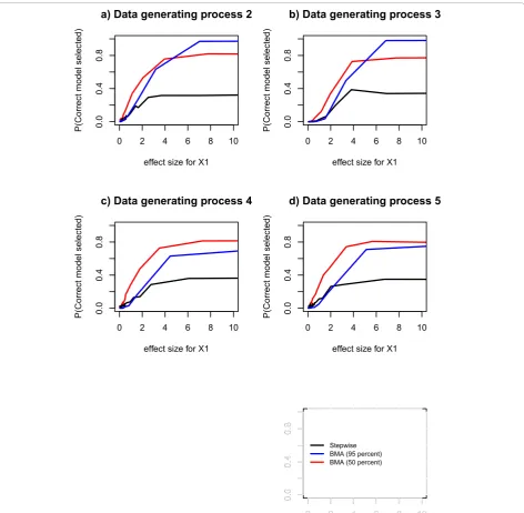
Probability of selecting correct model

The probability of selecting the correct model increased as the effect size of the true predictor increased but the

methods differed (Figure 4). Stepwise regression generally leveled out at selection probability approximately 0.3 in all data generating processes (Figure 4a-d). Bayesian model averaging with 95% threshold leveled out at approximately 1 for data generating processes 2 and 3 (Figure 4a and 4b) and on probability between 0.7 and 0.8 for data generating processes 4 and 5 (Figure 3c and 3d). Bayesian model aver-aging with 50% threshold leveled out at approximately 0.8 in all data generating processes (Figure 4a-d).

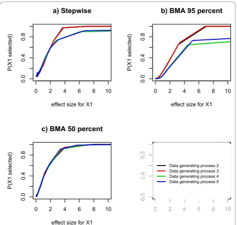
Influence of model complexity on selection probabilities

For data generating processes 4 and 5, the probability of selecting a true predictor in stepwise regression leveled out at a probability of approximately 0.9 compared to a probability of approximately 1 for data generating pro-cesses 2 and 3 (Figure 5a). In Bayesian model averaging with 95% threshold the probability of selecting a true predictor leveled out at a probability of approximately between 0.6 and 0.7 for data generating processes 4 and 5 compared to a probability of approximately of approximately 1 for data generating processes 2 and 3 (Figure 5b). In Bayesian model averaging with 50% threshold the probability of selecting a true predictor leveled out at 1 for all data generating processes (Figure 5c).

Discussion

threshold. Since the convention in the Bayesian model averaging literature is to use 50% posterior probability as a threshold, we focus discussion on comparison between stepwise regression and Bayesian model aver-aging with 50% posterior probability threshold.

Our notion that Bayesian model averaging is less likely than stepwise regression to select redundant variables is consistent with two previously published simulation stu-dies. In a study [8] with 10 simulations corresponding

to our data generating processes 1 and 3, Wang and col-leagues found Bayesian model averaging was less likely to select redundant variables than stepwise regression backward elimination. Despite differences in the study designs (logistic vs. linear regression and fewer simula-tions) their results are consistent with ours in support-ing the notion that Bayesian model averagsupport-ing is less likely to select redundant variables than stepwise regres-sion. Viallefont and coworkers performed a similar

0 2 4 6 8 10

0.6

0.7

0.8

0.9

1.0

a) Data generating process 2

effect size for X1

P(X3 not selected)

0 2 4 6 8 10

0.6

0.7

0.8

0.9

1.0

b) Data generating process 3

effect size for X1

P(X3 not selected)

0 2 4 6 8 10

0.6

0.7

0.8

0.9

1.0

c) Data generating process 4

effect size for X1

P(X3 not selected)

0 2 4 6 8 10

0.6

0.7

0.8

0.9

1.0

d) Data generating process 4

effect size for X1

P(X2 not selected)

0 2 4 6 8 10

0.6

0.7

0.8

0.9

1.0

e) Data generating process 5

effect size for X1

P(X3 not selected)

0 2 4 6 8 10

0.0

0.4

0.8

Stepwise BMA (95 percent) BMA (50 percent)

0 2 4 6 8 10

0.0

0.4

0.8

0 2 4 6 8 10

0.

00

.4

0.

8

study [15], based on 200 simulations, providing further support. They simulated data from a data generating process similar to our number 4 except with 50 vari-ables of which 10 were true predictions and some corre-lated with each other. Making use of stepwise regression backward elimination, they fitted logistic regression models and reported their results in terms of the pro-portion of selected variables that were true predictors.

They found stepwise regression more likely to select redundant variables than Bayesian model averaging. Of the variables selected (in the p-value intervals < 0.001, 0.001-0.01 and 0.01-0.05) by stepwise regression, 86% of them were true predictors whereas 98% were true among those selected by Bayesian model averaging (in the posterior probability intervals 95-99% and > 99%). Since those variables selected by Bayesian model

0 2 4 6 8 10

0.0

0.4

0.8

a) Data generating process 2

effect size for X1

P(X1 selected)

0 2 4 6 8 10

0.0

0.4

0.8

b) Data generating process 3

effect size for X1

P(X1 selected)

0 2 4 6 8 10

0.0

0.4

0.8

c) Data generating process 4

effect size for X1

P(X1 selected)

0 2 4 6 8 10

0.0

0.4

0.8

d) Data generating process 5

effect size for X1

P(X1 selected)

0 2 4 6 8 10

0.0

0.4

0.8

e) Data generating process 5

effect size for X1

P(X2 selected)

0 2 4 6 8 10

0.0

0.4

0.8

Stepwise BMA (95 percent) BMA (50 percent)

0 2 4 6 8 10

0.0

0.4

0.8

0 2 4 6 8 10

00

04

08

averaging contained a lower proportion of false posi-tives, we can conclude that the probability of selecting a redundant variable was lower for Bayesian model aver-aging than for stepwise regression. A study by Raftery and coworkers [2] also supports this conclusion. They simulated 50 standard normal redundant variables not related to a standard normal outcome variable, repeated the simulation 10 times and found that “In five simula-tions, Occam’s window chose only the null model. For the remaining simulations, three models or fewer were

chosen along with the null model”. On the other hand

“stepwise method chose models with many predictors”. In an earlier paper [13] Raftery and coworkers made a similar experiment which gave a similar result. In our study, we note that stepwise regression selected a redun-dant variable which correlates with a true predictor more often than it selected an uncorrelated variable, whereas Bayesian model averaging did not select a redundant variable even if it was correlated with a true predictor. The studies mentioned above [2,8,15] did not

0 2 4 6 8 10

0.0

0.4

0.8

a) Data generating process 2

effect size for X1

P(Correct model selected)

0 2 4 6 8 10

0.0

0.4

0.8

b) Data generating process 3

effect size for X1

P(Correct model selected)

0 2 4 6 8 10

0.0

0.4

0.8

c) Data generating process 4

effect size for X1

P(Correct model selected)

0 2 4 6 8 10

0.0

0.4

0.8

d) Data generating process 5

effect size for X1

P(Correct model selected)

0 2 4 6 8 10

0.0

0.4

0.8

Stepwise BMA (95 percent) BMA (50 percent)

0 2 4 6 8 10

0.0

0.4

0.8

0 2 4 6 8 10

0.

00

.4

0.

8

present probabilities of selecting a correlated redundant variable but Bayesian Model averaging is known to favor smaller models [16] and this supports our notion that Bayesian Model averaging is less likely than stepwise regression to select a redundant variable, be it uncorre-lated or correuncorre-lated with a true predictor.

The study by Wang and coworkers [8] also compared the probabilities of selecting a true predictor. In that work, both Bayesian model averaging and stepwise regression selected the two true predictors 10 out of 10 times. The study by Raftery and coworkers [2] provide some further support for the finding that Bayesian model averaging has a similar probability of selecting a true predictor as stepwise regression. Raftery and cowor-kers simulated a data set with one true predictor and 29 redundant variables. Occam’s window chose the correct model. Stepwise regression chose a model with two vari-ables - the true predictor together with a redundant variable. In the earlier study [13] Raftery and coworkers made two simulations of an outcome variable dependent on one true predictor but not related to 49 redundant variables. Both stepwise regression and Occam’s window selected the true predictor. Our study, with 300 simula-tions, shows that Bayesian model averaging with a pos-terior probability threshold of 50% has a similar probability of selecting a true predictor as stepwise regression. Available data thus show that the higher

probability of not selecting a redundant variable in Baye-sian model averaging compared to stepwise regression does not come at the price of lower probability of selecting a true predictor but instead provides us with similar probability of selecting a true predictor as step-wise regression. Bayesian model averaging almost never selected an indirect predictor, whereas stepwise regres-sion did, depending on effect size. Neither the Wang study [8] nor the study [15] by Viallefont presented probabilities of selecting an indirect predictor. The dif-ference between stepwise regression and Bayesian model averaging in selecting an indirect predictor was similar to the difference between the methods in the case with selection of the correlated redundant variable. This is not surprising since the two phenomena (selecting a correlated redundant variable and selecting an indirect predictor) are mathematically similar. Yamashita and colleagues [12] have given theoretical arguments and recommend that two highly correlated variables should not be entered into a selection procedure at the same time. Ideally, one of them should, based on subject mat-ter knowledge, be chosen.

The probability of selecting the correct model was substantially lower for stepwise regression than for Bayesian model averaging. The Wang study [8] reported that Bayesian model averaging selected the correct model 9 out of 10 times whereas stepwise regression only did 3 times out of 10. We do not, in our study, see a clear picture when comparing the probabilities of selecting the correct model in Bayesian model averaging with 95% and Bayesian model averaging with 50%. How-ever, based on available information we can conclude that Bayesian model averaging performs better than stepwise regression in selecting the correct model.

While Bayesian model averaging was primarily devel-oped as a method for model averaging and handling model uncertainty, we chose to explore the use of Baye-sian model averaging as a model selection method. Kass and Raftery [9] offer informative thresholds for interpret-ing posterior probabilities, providinterpret-ing us with the conven-tion that the posterior probability threshold 50% corresponds to the 0.05 p-value significance level. In our simulation study we use linear regression because it allowed us to directly control the variance independently of the regression coefficient and thus to control the effect size. We regard this as a strength of this study since none of the previously published studies comparing Bayesian model averaging and stepwise regression presented results for different values of the effect size. With our simulations we tried to mirror simple data generating processes that can be said to be basic components of what one encoun-ters in medical research. We deliberately chose data gener-ating processes that were small and simple in order to more easily see differences between the model selection

0 2 4 6 8 10

0.0

0.4

0.8

a) Stepwise

effect size for X1

P(X1 selected)

0 2 4 6 8 10

0.0

0.4

0.8

b) BMA 95 percent

effect size for X1

P(X1 selected)

0 2 4 6 8 10

0.0

0.4

0.8

c) BMA 50 percent

effect size for X1

P(X1 selected)

● ●

0 2 4 6 8 10

0.0

0.4

0.8

Data generating process 2 Data generating process 3 Data generating process 4 Data generating process 5

0 2 4 6 8 10

0.0

0.4

0.8

0 2 4 6 8 10

methods. Also, using a real life data set would not allow variation of the effect size. We view our chosen data gen-erating processes as the basic building blocks of what one encounters in real life, although recognize that the findings from our simple scenarios may not translate perfectly to real life. There is also a need for a more nuanced covar-iance structure. In our study, the probabilities of not selecting a redundant variable, not correlated with a true predictor, in both stepwise regression and Bayesian model averaging are approximately constant over changes in complexity of the data generating process. For stepwise regression, however, the probabilities of selecting a true predictor are higher for lower complexity of the data gen-erating process and gradually decrease with increasing complexity, whereas the probabilities of selecting a true predictor in Bayesian model averaging with 50% posterior probability threshold does not show this sensitivity to increasing complexity. If this advantage of Bayesian model averaging should persist even in the most complex real life data structures, it would add to the evidence in favor of Bayesian model averaging. This aspect deserves more attention and could be the topic of a future study of these methods.

Conclusion

Our simulation study showed that under the given con-ditions, Bayesian model averaging had a higher probabil-ity of not selecting a redundant variable than stepwise regression and had a similar probability of selecting a true predictor. Medical researchers building regression models with limited subject matter knowledge could thus benefit from using Bayesian model averaging.

Appendix

Bayesian model averaging

As described by Hoeting and coworkers [1], instead of basing inference on one single model, Bayesian model averaging takes into account all the models considered. For some quantity of interest θ, such as a regression coefficient, the inference aboutθ is not only based on one single selected model but on the average of all pos-sible models. For the quantity of interestθthe posterior distribution given data D is

p D p M D p M D

k K

k k

( | ) = ( | , ) ( | )

=

∑

This is an average of the posterior distributions under each of the K models considered - a sum of terms where each term is the posterior θ-probability given dataDand a modelMk, weighted by the probability for that modelMkgiven dataD.

So inference aboutθ is not only based on one single selected model but on an average of posterior

distributions of all identified models. In this way Baye-sian model averaging accounts for model uncertainty. In (1) the posterior probability for modelMkis given by

p M D p D M p M

p D M p M

k k k

l K

l l

( | ) ( | ) ( ) ( | ) ( )

=

=

∑

(2)

where

p D M( | k)=

∫

is the integrated likelihood of modelM_k,ξk is the vec-tor of parameters of model M_k, p(ξk|M_k) is the prior density ofξkunder modelM_k, p(D|ξk),M_kis the likeli-hood andp(M_k) is the prior probability that M_k is the true model.

The sum in (1) can be exhaustive. An approach for managing the summation is to average over a subset of models that are supported by data. One method for this is called the Occam’s window [17].

This is a method of accepting the models which are most likely to be the true model and not accepting any unnecessarily complicated model. Two principles that form the basis for the method are briefly presented here.

1. When comparing two models, the one that predicts data far less well than the better model should no longer be considered. A more formal way of saying this is that models not belonging to the setS1, where

S M p M D

p M D C

k l l

k

1={ :max { ( | )}≤

( | ) } (4)

should be excluded from (1).Cis chosen by the data analyst.

2. If a model is simpler or smaller than a model it is being compared with and data provides evidence for the simpler model, then the more complex model should no longer be considered. Thus models should also be excluded if they belong to the setS2, where

S M M S M M p M D

p M D

k l l k l

k

2={ :∃ ∈ 1, ⊂ , ( | ) >1 ( | ) } (5)

Then (1) is replaced by

p D p M D p M D

Mk S

k k

( | ) = ( | , ) ( | ),

∈

∑

now in the Bayesian model averaging literature is not to use the second principle.

The BMA package in R [11] is an implementation of the Bayesian model averaging method.

Acknowledgements

The authors would like to thank the reviewers, and in particular Professor Adrian E Raftery, who gave very helpful comments on the manuscript. This study was supported by Sahlgrenska Academy and Western Region of Sweden; contract/grant number: 98-1846389.

Author details

1_{Clinical Cancer Epidemiology, Department of Oncology, Institute of Clinical} Sciences, Sahlgrenska University Hospital, Gothenburg, Sweden.2_Clinical Cancer Epidemiology, Karolinska Institutet, Karolinska University Hospital, Stockholm, Sweden.3_{Department of Medical Epidemiology and Biostatistics,} Karolinska Institutet, Stockholm, Sweden.

Authors’contributions

AG and PD conceived the study. AG participated in its design, carried out its implementing and drafted the first version of the manuscript. PD

participated in study design. SzN participated in study implementation. GS and PD coordinated the study. All authors contributed to the writing and approved the final version.

Competing interests

The authors declare that they have no competing interests.

Received: 15 June 2010 Accepted: 6 December 2010 Published: 6 December 2010

References

1. Hoeting JA, Madigan D, Raftery AE, Volinsky CT:Bayesian Model Averaging: A Tutorial.Statistical Science1999,14:382-417.

2. Raftery AE, Madigan D, Hoeting JA:Bayesian Model Averaging for Linear Regression Models.Journal of the American Statistical Association1997, 92(437):179-191 [http://www.jstor.org/stable/2291462].

3. Harrell FEJ:Regression Modeling StrategiesSpringer; 2001.

4. Mundry R, Nunn CL:Stepwise model fitting and statistical inference: turning noise into signal pollution.Am Nat2009,173:119-123. 5. Greenland S:Modeling and Variable Selection in Epidemiologic Analysis.

American Journal of Public Health1989,79:340-349.

6. Malek MH, Berger DE, Coburn JW:On the inappropriateness of stepwise regression analysis for model building and testing.Eur J Appl Physiol

2007,101(2):263-4, author reply 265-6.

7. Pace NL:Independent predictors from stepwise logistic regression may be nothing more than publishable P values.Anesth Analg2008, 107(6):1775-1778.

8. Wang D, Zhang W, Bakhai A:Comparison of Bayesian model averaging and stepwise methods for model selection in logistic regression.

Statistics in Medicine2004,23:3451-3467.

9. Kass RE, Raftery AE:Bayes Factors.Journal of the American Statistical Association1995,90:773-795.

10. Jeffreys H:Theory of Probability.3 edition. Oxford, U.K.: Clarendon Press; 1961.

11. R Development Core Team:R: A Language and Environment for Statistical ComputingR Foundation for Statistical Computing, Vienna, Austria; 2010 [http://www.R-project.org], [ISBN 3-900051-07-0].

12. Yamashita T, Yamashita K, Kamimura R:A Stepwise AIC Method for Variable Selection in Linear Regression.Communications in Statistics: Theory & Methods2007,36(13):2395-2403 [http://search.ebscohost.com/ login.aspx?direct=true&db=buh&AN=26774447&site=ehost-live]. 13. Raftery AE:Bayesian model selection in social research.Sociological

Methodology1995,25:111-163.

14. Raftery AE, Painter IS, Volinsky CT:BMA: An R package for Bayesian Model Averaging.R News2005,5(2):2-8 [http://CRAN.R-project.org/doc/Rnews/]. 15. Viallefont V, Raftery AE, Richardson S:Variable selection and Bayesian

model averaging in case-control studies.Statistics in Medicine2001, 20(21):3215-3230.

16. Yang Y:Can the strengths of AIC and BIC be shared? A conflict between model indentification and regression estimation.Biometrika2005, 92(4):937-950 [http://biomet.oxfordjournals.org/cgi/content/abstract/92/4/ 937].

17. Madigan D, Raftery AE:Model Selection and Accounting for Model Uncertainity in Graphical Models Using Occam_’s Window.Journal of the American Statistical Association1994,89:1535-1546, [Pdf].

Pre-publication history

The pre-publication history for this paper can be accessed here: http://www.biomedcentral.com/1471-2288/10/108/prepub

doi:10.1186/1471-2288-10-108

Cite this article as:Genellet al.:Model selection in Medical Research: A simulation study comparing Bayesian Model Averaging and Stepwise Regression.BMC Medical Research Methodology201010:108.

Submit your next manuscript to BioMed Central and take full advantage of:

• Convenient online submission

• Thorough peer review

• No space constraints or color figure charges

• Immediate publication on acceptance

• Inclusion in PubMed, CAS, Scopus and Google Scholar

• Research which is freely available for redistribution