AUTOMATIC ESTIMATION OF ICE BOTTOM SURFACES FROM RADAR IMAGERY

AUTOMATIC ESTIMATION OF ICE BOTTOM SURFACES FROM RADAR IMAGERY

Mingze Xu

David J. Crandall

Geoffrey C. Fox

John D. Paden

†

_{School of Informatics and Computing, Indiana University, Bloomington, IN USA}

⋆

_{Center for Remote Sensing of Ice Sheets, University of Kansas, Lawrence, KS USA}

ABSTRACT

Ground-penetrating radar on planes and satellites now makes it practical to collect 3D observations of the subsurface struc-ture of the polar ice sheets, providing crucial data for under-standing and tracking global climate change. But convert-ing these noisy readconvert-ings into useful observations is generally done by hand, which is impractical at a continental scale. In this paper, we propose a computer vision-based technique for extracting 3D ice-bottom surfaces by viewing the task as an inference problem on a probabilistic graphical model. We first generate a seed surface subject to a set of constraints, and then incorporate additional sources of evidence to refine it via dis-crete energy minimization. We evaluate the performance of the tracking algorithm on 7 topographic sequences (each with over 3000 radar images) collected from the Canadian Arctic Archipelago with respect to human-labeled ground truth.

Index Terms— Glaciology, Radar tomography, 3D re-construction, Graphical models

1. INTRODUCTION

Scientists increasingly use visual observations of the world in their work: astronomers collect telescope images at unprece-dented scale [1], biologists image live cells [2, 3], sociologists record social interactions [4], ecologists collect large-scale re-mote sensing data [5], etc. Although progress in technology

has madecollecting this imagery affordable, actually

ana-lyzingit is often done by hand. But with recent progress in computer vision, automated techniques may soon work well enough to remove this bottleneck, letting scientists analyze visual data more thoroughly, quickly, and economically.

As a particular example, glaciologists need large-scale data about the polar ice sheets and how they are changing over time in order to understand and predict the effects of melting glaciers. Aerial ground-penetrating radar systems have been developed that can fly over an ice sheet and collect evidence about its subsurface structure. The raw radar re-turn data is typically mapped into 2D radar echogram images which are easier for people to interpret, and then manually labeled for important semantic properties (ice thickness and structure, bedrock topography, etc.) in a slow, labor-intensive process [6, 7, 8, 9]. Some recent work has shown

promis-ing results on the specific problem of layer-findpromis-ing in 2D echograms [10, 11, 12], although the accuracy is still far be-low that of a trained human annotator. The echograms are usually quite noisy and complex, requiring experience and intuition that is difficult to encode in an algorithm. Using echograms as input data also inherently limits the analysis to the ice structure immediately under the radar’s flight path.

In this paper we take an alternative approach, using ad-ditional data collected by the radar in order to actually esti-mate the 3D structure of the ice sheet, including a large area on either side, instead of simply tracing 2D cross-sections (Figure 1). In particular, the Multichannel Coherent Radar Depth Sounder (MCoRDS) instrument [13] uses three trans-mit beams (left, nadir, right) to collect data from below the airplane and to either side (for a total swath width of about 3km). Although an expert may be able to use intuition and experience to produce a reasonable estimate of the 3D ter-rain from this data, the amount of weak evidence that must be considered at once is overwhelming. As with structure-from-motion in images [14], this gives automatic algorithms an ad-vantage: while humans are better at using intuition to estimate from weak evidence, algorithms can consider a large, hetero-geneous set of evidence to make better overall decisions.

We formulate the problem as one of discrete energy min-imization in order to combine weak evidence into a 3D re-construction of the bottom of the ice sheet. We first estimate layer boundaries to generate a seed surface, and then incorpo-rate additional sources of evidence, such as ice masks, surface digital elevation models, and optional feedback from humans to refine it. We investigate the performance of the algorithm using ground truth from humans, showing that our technique significantly outperforms several strong baselines.

2. RELATED WORK

Detecting boundaries between material layers in noisy radar

images is important for glaciology. Semi-automated and

automated methods have been introduced for identifying

fea-tures of subsurface imaging. For example, in echograms

Fig. 1. Illustration of our task. Radar flies along the X-axis, collecting noisy evidence about the ice surface distance and depth immediately below it. This yields a 2D echogram (Sample (c)), with depth on one axis and flight path on the other, and prior work has used these echograms to estimate 2D ice structure but only along the flight path. Our approach also includes (very noisy) evidence from either side of the radar, yielding a sequence of 2D topographic slices (e.g. Sample (a) and (b)). Each slice is represented in polar coordinates, where Y- and Z-axis denote the direction of arrival of radar waves and the distance from each voxel to plane, respectively. We combine this noisy evidence with prior information to produce 3D ice reconstructions.

specific case of ice, Crandall et al. [10] detect the ice-air and ice-bottom layers in echograms along the flight path by com-bining a pretrained template model for the vertical profile of each layer and a smoothness prior in a probabilistic graphical model. Lee et al. [11] present a more accurate technique that uses Gibbs sampling from a joint distribution over all possible layers. Carrer and Bruzzone [12] reduce computational com-plexity with a divide-and-conquer strategy. In contrast to the above work which all infers 2D cross-sections, we attempt to reconstruct 3D subsurface features and are not aware of other work that does this. We pose this as an inference problem on a Markov Random Field similar to that proposed for vision problems (e.g. stereo [16]), except that we have a large set of images and wish to produce a 3D surface, whereas they perform inference on a single 2D image at a time.

3. METHODOLOGY

As the radar system flies over ice, it collects a sequence of

topographic slicesI={I1,· · · , Il}that characterizes the

re-turned radar signals (Figure 1). Each sliceIi is a 2D radar

image that describes a distribution of scattered energy in

po-lar coordinates (with dimensionsφ×ρ)at a discrete position

iof the aircraft along its flight path. Given such a topographic

sequence of dimensionl×φ×ρ, we wish to infer the 3D

ice-bottom surface. We parameterize the surface as a sequence

of slicesS={S1,· · ·, Sl}andSi ={si,1,· · ·, si,φ}, where

si,j denotes the row coordinate of the boundary of the

ice-bottom for columnj of slice i, andsi,j ∈ [1, ρ] since the

ice-bottom layer can occur anywhere within a column.

3.1. A graphical model for surface extraction

Because radar is so noisy, our goal is to find a surface that not only fits the observed data well but that is also smooth and satisfies other prior knowledge. We formulate this as an inference problem on a Markov Random Field. In particular,

we look for a surface that minimizes an energy function,

E(S|I) =

l X

i=1

φ X

j=1

ψ1(si,j|I) + (1)

l X

i=1

φ X

j=1

X

i′∈±1

X

j′∈±1

ψ2(si,j, si+i′,j+j′) (2)

where ψ1(·) defines a unary cost function which measures

how well a given labeling agrees with the observed image

inI, andψ2(·,·)defines a pairwise interaction potential on

the labeling which encourages the surface to be continuous and smooth. Note that each column of each slice contributes one term to the unary part of the energy function, while the pairwise terms are a summation over the four neighbors of a column (two columns on either side within the same slice, and two slices within the same column in neighboring slices).

Unary term.Our unary termψ1(·)consists of three parts,

ψ1(·) =ψtemp_{(·) +ψ}air_{(·) +ψ}bin_(·).

(3)

First, similar to [10], we define a template modelT of fixed

size1×t(we uset= 11pixels) for the vertical profile of the

ice-bottom surface in each slice. For each pixelpin the

tem-plate, we estimate a meanµpand a varianceσpon greyscale

intensity assuming that the template is centered at the location of the ice-bottom surface, suggesting a template energy,

ψtemp_(s i,j|I) =

X

p∈T

(I(si,j+p)−µp)

2

/σp. (4)

We learn the parameters of this model with a small set of la-beled training data.

Error Precision

Mean Median Mean 1 pixel 5 pixels

(a) Ice-bottom surfaces:

Crandall [10] 101.6 95.9 0.2% 2.5% Lee [11] 35.6 30.5 3.6% 29.9% Ours withDV 13.3 13.4 20.2% 58.3% Ours withTRW 11.9 12.2 35.9% 63.9%

(b) Bedrock layers:

Crandall [10] 75.3 42.6 0.5% 21.5% Lee [11] 47.6 36.6 2.2% 20.5% Ours withTRW 4.1 4.2 28.8% 81.4%

Table 1. Error in terms of the mean and median mean ab-solute column-wise difference compared to ground truth, in pixels. Precision is the percentage of correct labeled pixels.

margin, we add a cost to penalize intersecting surfaces,

ψair(sij) = 

 

 

+∞ si,j−ai,j<0

0 si,j−ai,j> τ

τ− |si,j−ai,j| otherwise,

(5)

withai,jthe label of the air-ice boundary of slicei, columnj.

Finally, we incorporate an additional weak source of

evi-dence produced by the radar system. Thebottom bingives a

constraint on asinglecolumn in each slice, specifying a

sin-gle coordinate(j, bi)that the true surface boundary must be

below. Despite how weak this evidence is, it helps to distin-guish between the ice-air and ice-bottom surface boundary in practice. Formally, we formulate this cost function as,

ψbin(si,j) = (

+∞ si,j< bi

0 otherwise. (6)

Pairwise term. The ice-bottom surface is encouraged to be smooth across both adjacent columns and adjacent slices,

ψ2(s,ˆs) =

(

−βjlnN(s−ˆs; 0,σˆ) |s−sˆ|< α

+∞ otherwise, (7)

whereˆsdenotes the labeling of an adjacent pixel of (i, j), and

parametersαandσˆ are learned from labeled training data.

Parameterβjmodels smoothness on a per-slice basis, which

is helpful if some slices are known to be noisier than others (or set to a constant if this information is not known). This term models the similarity of the labeling of two adjacent pixels by a zero-mean Gaussian that is truncated to zero outside a fixed

interval α. Since all parameters in the energy function are

considered penalties, we transform the Gaussian probability to a quadratic function by using a negative logarithm.

Our energy function introduces several important im-provements over that of Crandall et al. [10] and Lee et al. [11]. First, while their model gives all pairs of adjacent pixels the

500 1000 1500 2000 2500 3000 10

20

30

40

50

60 Ground truth

500 1000 1500 2000 2500 3000 10

20

30

40

50

60 Result of [11]

500 1000 1500 2000 2500 3000 10

20

30

40

50

60 Ours with DV

500 1000 1500 2000 2500 3000 10

20

30

40

50

60 Ours with TRW

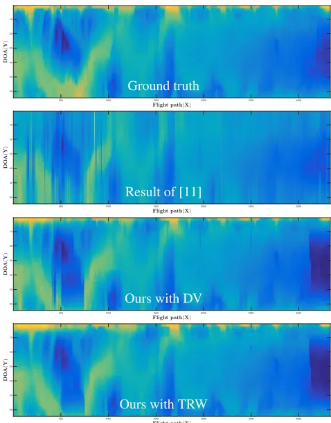
Fig. 2. Results of the ice-bottom surface finding on a sample dataset. The color represents the depth from plane (Z).

same pairwise weight (β), we have observed that layers in

different slices usually have particular shapes, such as straight lines and parabolas, depending on the local ice topography.

By using a dynamic weightβj, we can roughly control the

shape of the layer and adjust how smooth two adjacent pixels should be. More importantly, those techniques consider a single image at a time, which could cause discontinuities in the ice reconstruction. We correct this by defining pairwise terms along both the intra- and inter-slice dimensions.

3.2. Statistical inference

The minimization of equation (1) can be formulated as

Ground truth

Result of [10]

Result of [11]

Ours with TRW

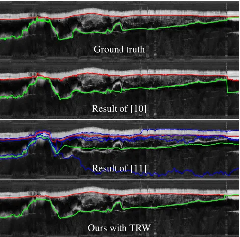
Fig. 3. Results of the bedrock layer finding on a sample echogram. In each image, the upper (red) boundary is the ice-air layer, and the lower (green) boundary is the ice-bottom layer. The ice-air layer in our result is from the radar.

order. We pre-define a maximum number of iterations to be

the same as the width of each slice,φ, which allows evidence

from one side of the slice to be reach the other. When mes-sage passing is finished, we assign a label to each pixel in

row-major order: for pixel(i, j), we choose the labelsi,jthat

minimizesψ1(si,j) +ψ2(si,j, si,j−1) +ψ2(si,j, si−1,j).

The usual implementation of TRW has time complexity

O(lφρ2₎

for each loop. To speed this up, we use linear-time generalized distance transforms [16], yielding a total running

time ofO(lφρL)whereLis the number of iterations. This is

possible because of our pairwise potentials are log-Gaussian.

4. EXPERIMENTS

We tested our surface extraction algorithm on the basal topog-raphy of the Canadian Arctic Archipelago (CAA) ice caps, collected by the Multichannel Coherent Radar Depth Sounder (MCoRDS) instrument [13]. We used a total of 7 topographic sequences, each with over 3000 radar images which corre-sponds to about 50km of flight data per sequence. For these images, we also have the associated ice-air surface ground truth, a subset (excluded from the testing data) of which we used to learn the parameters of the template model and the weights of the binary costs.

We then ran inference on each topographic sequence and measured the accuracy by comparing our estimated surfaces to the ground truth, which was produced by human annota-tors. However, these labels are not always accurate at the pixel-level, since the radar images are often full of noise, and

some boundaries simply cannot be tracked precisely even by experts. To relax the effect of inaccuracies in ground truth, we consider a label to be correct when it is within a few pix-els. We evaluated with three summary statistics: mean devi-ation, median mean devidevi-ation, and the percentage of correct labeled pixels over the whole surface (Table 1(a)). The mean error is about 11.9 pixels and the median-of-means error is about 12.2 pixels. The percentage of correct pixels is 35.9%, or about 63.9% within 5 pixels, which we consider the more meaningful statistic given noise in the ground truth.

To give some context, we compare our results with three baselines. Since no existing techniques solve the 3D recon-struction problem that we consider here, we adapted three techniques from 2D layer finding to the 3D case. Crandall et al. [10] use a fixed weight for the pairwise conditional probabilities in the Viterbi algorithm, which cannot automat-ically adjust the shape of the layer in each image slice. Lee et al. [11] generate better results by using Markov-Chain Monte Carlo (MCMC). However, neither of these approaches con-siders constraints between adjacent slices. We introduce Dy-namic Viterbi (DV) as an additional baseline that incorporates a dynamic weight for the pairwise term, but it still lacks the ability to smooth the whole surface in 3D. As shown in Table 1(a) and Figure 2, our technique performs significantly better than any of these baselines on 3D surface reconstruction. We also used our technique to estimate layers in 2D echograms, so that we could compare directly to the published source code of [10, 11] (i.e. using our approach to solve the prob-lem they were designed for). Figure 3 and Table 1(b) present results, showing a significant improvement over these base-lines also.

Similar to [10, 11], additional evidence can be easily added into our energy function. For instance, ground truth data (e.g. ice masks) may be available for some particular slices, and human operators can also provide feedback by marking true surface boundaries for a set of pixels. Either of these can be implemented by putting additional terms into the

unary term defined in equation (3).

5. CONCLUSION

To the best of our knowledge, this paper is the first to propose an automated approach to reconstruct 3D ice features using graphical models. We showed our technique can effectively estimate ice-bottom surfaces from noisy radar observations. This technique also demonstrated its accuracy and efficiency in producing bedrock layers on radar echograms against the state-of-the-art.

6. ACKNOWLEDGEMENTS

7. REFERENCES

[1] Alexander Szalay and Jim Gray, “The world-wide

tele-scope,” Science, vol. 293, no. 5537, pp. 2037–2040,

2001.

[2] Jyoti K Jaiswal, Hedi Mattoussi, J Matthew Mauro, and Sanford M Simon, “Long-term multiple color imaging

of live cells using quantum dot bioconjugates,” Nature

Biotechnology, vol. 21, no. 1, pp. 47–51, 2003.

[3] David J Stephens and Victoria J Allan, “Light

mi-croscopy techniques for live cell imaging,”Science, vol.

300, no. 5616, pp. 82–86, 2003.

[4] Claus Wedekind and Manfred Milinski, “Cooperation

through image scoring in humans,” Science, vol. 288,

no. 5467, pp. 850–852, 2000.

[5] Jonathan Bamber, Jennifer Griggs, Ruud Hurkmans, Ju-lian Dowdeswell, Prasad Gogineni, Ian Howat, Jeremie Mouginot, John Paden, Steven Palmer, Eric Rignot,

et al., “A new bed elevation dataset for greenland,” The

Cryosphere, vol. 7, no. 2, pp. 499–510, 2013.

[6] Greg J Freeman, Alan C Bovik, and John W Holt, “Au-tomated detection of near surface martian ice layers in

orbital radar data,” inSouthwest Symposium on Image

Analysis & Interpretation (SSIAI), 2010, pp. 117–120.

[7] Ana-Maria Ilisei, Adamo Ferro, and Lorenzo Bruzzone, “A technique for the automatic estimation of ice thick-ness and bedrock properties from radar sounder data

ac-quired at Antarctica,” inInternational Geoscience and

Remote Sensing Symposium (IGARSS), 2012, pp. 4457– 4460.

[8] Adamo Ferro and Lorenzo Bruzzone, “Automatic ex-traction and analysis of ice layering in radar sounder

data,” IEEE Transactions on Geoscience and Remote

Sensing, vol. 51, no. 3, pp. 1622–1634, 2013.

[9] Jerome E Mitchell, David J Crandall, Geoffrey C Fox, and John D Paden, “A semi-automatic approach for esti-mating near surface internal layers from snow radar

im-agery,” inInternational Geoscience and Remote Sensing

Symposium (IGARSS), 2013, pp. 4110–4113.

[10] David J Crandall, Geoffrey C Fox, and John D Paden, “Layer-finding in radar echograms using probabilistic

graphical models,” inInternational Conference on

Pat-tern Recognition (ICPR), 2012, pp. 1530–1533.

[11] Stefan Lee, Jerome Mitchell, David J Crandall, and Ge-offrey C Fox, “Estimating bedrock and surface layer boundaries and confidence intervals in ice sheet radar

imagery using MCMC,” inInternational Conference on

Image Processing (ICIP), 2014, pp. 111–115.

[12] Leonardo Carrer and Lorenzo Bruzzone, “Automatic enhancement and detection of layering in radar sounder data based on a local scale hidden Markov model and the

Viterbi algorithm,” IEEE Transactions on Geoscience

and Remote Sensing, vol. 55, no. 2, pp. 962–977, 2017.

[13] Fernando Rodriguez-Morales, Sivaprasad Gogineni, Carlton J Leuschen, John D Paden, Jilu Li, Cameron C

Lewis, Benjamin Panzer, Daniel Gomez-Garcia

Alvestegui, Aqsa Patel, Kyle Byers, et al., “Advanced multifrequency radar instrumentation for polar

re-search,” IEEE Transactions on Geoscience and Remote

Sensing, vol. 52, no. 5, pp. 2824–2842, 2014.

[14] David Crandall, Andrew Owens, Noah Snavely, and

Daniel Huttenlocher, “SfM with MRFs:

Discrete-continuous optimization for large-scale structure from

motion,” IEEE Transactions on Pattern Analysis and

Machine Intelligence, vol. 35, no. 12, pp. 2841–2853, 2013.

[15] Adamo Ferro and Lorenzo Bruzzone, “A novel approach to the automatic detection of subsurface features in

plan-etary radar sounder signals,” in IEEE International

Geoscience and Remote Sensing Symposium (IGARSS), 2011, pp. 1071–1074.

[16] Pedro F Felzenszwalb and Daniel P Huttenlocher,

“Effi-cient belief propagation for early vision,” International

Journal of Computer Vision, vol. 70, no. 1, pp. 41–54, 2006.

[17] Daphne Koller and Nir Friedman, Probabilistic

graphi-cal models: principles and techniques, 2009.

[18] Vladimir Kolmogorov, “Convergent tree-reweighted

message passing for energy minimization,”

Transac-tions on Pattern Analysis and Machine Intelligence, vol. 28, no. 10, pp. 1568–1583, 2006.

[19] Kevin P Murphy, Yair Weiss, and Michael I Jordan, “Loopy belief propagation for approximate inference:

An empirical study,” in Proceedings of the Fifteenth