CONTENT-BASED POPULARITY PREDICTION ON
SOCIAL MICROBLOGS
by Axel Magnuson
A thesis
submitted in partial fulfillment of the requirements for the degree of Master of Science in Computer Science
Boise State University
DEFENSE COMMITTEE AND FINAL READING APPROVALS
of the thesis submitted by
Axel Magnuson
Thesis Title: Evaluation of Topic Models for Content-Based Popularity Prediction on Social Microblogs
Date of Final Oral Examination: 17 December 2015
The following individuals read and discussed the thesis submitted by student Axel Magnuson, and they evaluated his presentation and response to questions during the final oral examination. They found that the student passed the final oral examination.
María Soledad Pera, Ph.D. Chair, Supervisory Committee Timothy Andersen, Ph.D. Member, Supervisory Committee Edoardo Serra, Ph.D. Member, Supervisory Committee
The author wishes to deeply thank Dr. Mar´ıa Soledad Pera and Dr. Vijay Dialani for their invaluable guidance in my degree. Special recognition is due to Dr. Mar´ıa Soledad Pera, whose exceptional effort in guiding this thesis went far above the call of duty. He would additionally like to thank the wonderful staff and faculty of Boise State University for their persistence and diligence in educating him, alongside his many colleagues. Among them, he wishes to name Dr. Amit Jain, Dr. Timothy Andersen, and Dr. Elena Sherman for their exceptional capacities as educators.
Furthermore, the author owes any of his achievement in life to the kind generosity of the those who have guided and supported him throughout his life. In particular, he would like to thank his Mother, Father, and Brother for their profound support and love. He would also like to thank a long line of inspiring teachers including David Pover, Tatia Totorica, AlejAndro Anastasio, and Dr. Arun Ram. The author wishes to acknowledge the incredible impact that all of those above have had on his life and their utter necessity in the production of this work. He owes thanks to the kind support of his many colleagues, especially Deepa Mallela, Nevena Dragovic, and Jim Pelton. Finally, he would like to thank Dr. Vijay Dialani and Dr. Edoardo Serra for their roles in providing the funding necessary to support the author throughout his endeavor.
Online social networks are an increasingly central medium of communication in the 21st century. We have seen a proliferation of competing social networks that differentiate themselves by serving different niches of communication. Among these, Twitter has risen to prominence as a leader among microblogging communities, characterized by publicly visible 140-character messages called tweets. The wide visibility of Twitter messages has enabled some users to curate large followings, and has facilitated content creators who wish to reach as many viewers as possible. Researchers have since investigated many methods for predicting which messages will become popular or even go viral on Twitter. Although there are many facets to this research problem, and various methods of approaching it have been proposed, we note that anyone who wants to create a popular Twitter account will sooner or later have to produce popular content. In this study, we investigated the content-based approach of predicting popular tweets based only on the text they contain. Particularly, we asked whether topic models can be used to identify topics of discussion that are more likely to be associated with popular tweets. In the process, we explored methods for collecting and processing a large-scale corpus of Twitter content. Our experiments found that while topic-based prediction methods could lead to effective popularity prediction, they were outperformed by other, simpler content-based methods.
ABSTRACT . . . vi
LIST OF TABLES . . . ix
LIST OF FIGURES . . . xi
LIST OF ABBREVIATIONS . . . xiii
1 Introduction . . . 1
1.1 Popularity Prediction and Influence Analysis . . . 2
1.2 Topic Models . . . 5
1.3 Research Aims . . . 7
2 Thesis Statement . . . 9
3 Dataset . . . 10
3.1 Twitter Statuses . . . 10
3.1.1 Twitter API . . . 11
3.1.2 Collection . . . 13
3.2 Processing Techniques . . . 14
3.2.1 Big Data . . . 15
3.2.2 Local Analysis . . . 22
4.1 Using Hashtags for Popularity Prediction . . . 24
4.2 Identifying the Topic Spaces of Hashtags . . . 32
4.2.1 Labeled Latent Dirichlet Allocation . . . 32
4.2.2 Token Correlation . . . 35
5 Direct Popularity Prediction with SLDA . . . 39
5.1 Parameter Selection for SLDA . . . 43
5.1.1 Sweep 1E5–1 . . . 44
5.1.2 Sweep 1E5–2 . . . 53
5.1.3 Sweep 1E5–3 . . . 63
5.2 SLDA Performance Analysis . . . 66
6 Conclusion . . . 71
6.1 Future Works . . . 72
REFERENCES . . . 74
A Computing Resources . . . 78
A.1 BDServer Hadoop Cluster . . . 78
A.2 Infolab . . . 78
A.3 Sweet Chedda . . . 79
3.1 Example Twitter REST Endpoint Rate Limits . . . 11
3.2 Twitter Streaming Endpoints . . . 12
3.3 Filter Limits on statuses/filter . . . 13
3.4 InfluenceFlow Dataset Statistics . . . 16
3.5 TClean Cleaning Steps . . . 18
3.6 TClean Cleaning Statistics . . . 20
4.1 pˆA Classification Performance . . . 27
4.2 pˆA Logistic Classifier Performance . . . 29
4.3 pˆB Clasification Performance . . . 31
4.4 pˆB Logistic Classifier Performance . . . 31
4.5 Summary of Hashtag Predictor Performance Metrics . . . 31
4.6 Run Times for LDA and LLDA tests . . . 35
4.7 pˆC Clasification Performance . . . 36
4.8 pˆC Logistic Classifier Performance . . . 36
4.9 Summary of Hashtag Predictor Performance Metrics . . . 37
5.1 Model Parameters for sLDA . . . 41
5.2 Estimation Parameters for sLDA . . . 44
5.3 Ranges for sLDA Sweep 1E5–1 . . . 45
5.4 Static Parameters for sLDA Sweep 1E5–1 . . . 46
5.6 Sweep 1E5–1 Dimensionality vs Timing Regression Results . . . 51
5.7 Ranges for sLDA Sweep 1E5–2 . . . 57
5.8 Pearson’s r Correlations of ˆLemk. . . 58
5.9 Static Parameters for sLDA Sweep 1E5–3 . . . 64
5.10 Ranges for sLDA Sweep 1E5–3 . . . 64
5.11 Tested Predictive Models . . . 67
5.12 Summary of Predictor Performance . . . 67
5.13 Popular Topics and Their Most Frequently Assigned Words . . . 70
A.1 BDServer Node System Specifications . . . 78
A.2 Infolab System Specifications . . . 79
A.3 SweetChedda System Specifications . . . 79
3.1 Daily Collection Volumes for 2014 through 2015 . . . 14
3.2 Effect of t1 Threshold on Remaining Word Count rVn on the domains t1 ∈[15,300] and t1 ∈[3×102,2×104] . . . 20
3.3 Effect of t1 Threshold on Remaining Document Count rDn on the do-mains t1 ∈[15,300], t1 ∈[3×102,2×104], and t1 ≥2×10⁴ . . . 21
4.1 pˆA Classification ROC Curve . . . 27
4.2 pˆA Logistic Classifier Visualization . . . 29
4.3 pˆA Logistic Classifier Receiver Operating Characteristic . . . 30
4.4 A Plate Notation Representation of LLDA [31] . . . 33
4.5 pˆC Logistic Classifier ROC Curve . . . 37
5.1 A Plate Notation Representation of sLDA [23] . . . 41
5.2 Sweep 1E5–1 Mean Log Loss and Mean Elapsed Time . . . 48
5.3 Error % of Sweep 1E5–1 Mean Log Loss and Mean Elapsed Time . . . 49
5.4 3σemk of Sweep 1E5–1 Mean Log Loss and Mean Elapsed Time . . . 50
5.5 Sweep 1E5–1 Dimensionality vs Timing Regression . . . 52
5.6 Sweep 1E5–1 Log Loss vs Elapsed Time . . . 54
5.7 Sweep 1E5–1 Log Loss vs Elapsed Time, Stratified by e,m, and k . . . . 55
5.8 Sweep 1E5–1 Log Loss vs Elapsed Time Split By k∈K . . . 56
5.9 Sweep 1E5–2 Mean Log Loss and Mean Elapsed Time . . . 59
5.11 3σemk of Sweep 1E5–2 Mean Log Loss and Mean Elapsed Time . . . 61
5.12 Dimensionality vs Log Loss for Sweep 1E5–2 . . . 62
5.13 m vs Log Loss for Sweep 1E5–2 . . . 62
5.14 k vs Log Loss for Sweep 1E5–2 . . . 63
5.15 k vs Log Loss for Sweep 1E5–3 . . . 65
5.16 sLDA Classification ROC Curve . . . 68
5.17 Multinomial Naive Bayes Classification ROC Curve . . . 68
5.18 Bernoulli Naive Bayes Classification ROC Curve . . . 69
5.19 Ensemble Logistic Classification ROC Curve . . . 69
AUC – ROC Area Under Curve
FPR– False Positive Rate
LDA – Latent Dirichlet Allocation
LLDA – Labeled Latent Dirichlet Allocation
OANC – Open American National Corpus
OSN – Online Social Network
PGM – Probabilistic Graphical Model
ROC – Receiver Operating Characteristic
sLDA – Supervised Latent Dirichlet Allocation
TFIDF – Term Frequency Inverse Document Frequency
TPR – True Positive Rate
UGC – User Generated Content
CHAPTER 1
INTRODUCTION
Over the past two decades, online social networks (OSNs) such as Twitter, Facebook, YouTube, and Instagram have established themselves as central institutions in the realm of human socialization and interpersonal communication. They have especially disrupted traditional media industries, making online media both more accessible to authors and more reliant on interpersonal connections for visibility [20]. User generated content (UGC) has seen great proliferation under this environment, leading to a flourishing of blogs, videos, and messages all highly interconnected through OSN platforms.
Of particular interest are microblogging platforms such as Twitter, which continue to see widespread adoption and have become active, vibrant communities for online interaction [18]. In the microblogging format, users form connections by “following” other accounts, and post short 140-character messages that are visible to their own followers. For the purposes of this thesis, these messages are also referred to inter-changeably as “tweets” or “statuses.”1 Any user may follow and interact with any other user, distinguishing Twitter from more closed social networks like Facebook, which require the “followee” to reciprocate the relationship before the users can interact.
The Twitter microblogging platform has gained particular prominence in the area of real-time news and citizen journalism. Partially due to its public format, UGC on Twitter has the potential to gain viral popularity and achieve far-reaching impact [20]. This also makes Twitter a convenient target for academic study, as the majority of its content is public and freely accessible. However, with messages limited to 140 characters or less, it also presents novel challenges for content-based approaches that rely on larger document lengths.
As microblogging gains traction, the value of becoming an influential participant has become increasingly apparent. Many participants use Twitter as a means to advance their business goals or public image, and treat it as more of a marketing vector than an avenue of self expression [26]. An influential Twitter account can be a highly valued asset for both businesses and individuals [26]. To this end, many users attempt to leverage microblog features, such as hashtags and follow reciprocation, in order to increase their own influence in the system. As microblogs guide more eyes to online content, the study of predicting popularity and influence has become increasingly valuable for the tasks of trend forecasting, studying social dynamics, and predicting real-world events [15]. These efforts commonly fall into the related fields of popularity prediction and influence analysis, both of which we draw from in this work.
1.1
Popularity Prediction and Influence Analysis
of retweets or favorites, or it could be the more abstract measure of an inferred force within a system. Across the surveyed papers, many different definitions of influence were proposed, using a wide variety of problem formulation. While early influence measures relied largely on relationship graphs between users [19], more recent work has begun to incorporate social media-specific features [9, 17, 37]. These later influence measures add value by offering greater and more specific predictive value than their predecessors. These works on influence analysis often conceptualize influence on a latent feature of users or communities, remaining relatively stable between individual messages [9, 17, 19].
Cha et al. made the famous observation that indegree, or number of followers, is not necessarily a good measure of user influence [11]. They measured influence by a user’s propensity to spawn retweets or mentions, and found that influence was gained through a deliberate effort by users, and involved limiting tweets to a single topic. This final point is particularly interesting from our perspective. It provides initial evidence that carefully crafting tweets towards topical content is indeed an effective method of building user influence.
Other approaches rely on more sophisticated structural measures than indegree. TwitterRank is one such paper that proposes a method of quantifying user influence using a modified PageRank algorithm [35]. While these user-based influence studies are somewhat tangential to our study, the methods they use to measure influence can inform our own influence metrics.
In Twitter, this most often takes the form of retweet events, although favorites and replies could also be considered [15, 16, 33]. These problem formulations are more straightforward, allowing researchers to more easily measure their results. In fact, papers on influence measurement have used popularity prediction as a benchmark to quantify the performance of novel methods [17].
Much of the underlying value of a message’s popularity comes from its wide visibility in a network. In fact, for all practical purposes, the visibility of a message and its popularity are equivalent. The primary mechanism by which messages gain visibility on Twitter is by being retweeted, where a user reposts another user’s content to their own followers in an attributed manner. In this way, the message reaches followers who may not have seen it originally. Similar additional exposure is given to messages that are favorited or replied to, but with somewhat different social implications. Current popularity prediction methods can be roughly segmented into two approaches. The first attempts to predict popularity as a traditional machine learning task, using various relevant features to make predictions about how much a message will be retweeted [8, 14–16]. Although many relevant factors and methods have been explored, this is still a large, open area of research. Due to the complexity and variability of OSN communities, it remains difficult to predict popularity from traditional tweet features. The second group of prediction methods instead investigate the time dynamics of retweets. By recognizing patterns of retweets over time early in a message’s lifecycle, they estimate the total popularity that the message can be expected to achieve [15, 32]. While this has led to effective results, and definitely informs us as to the process by which tweets gain popularity over time, it provides very little information as to the causative factors of a message’s popularity.
such as hashtags, URLs, and number of friends and followees have all been shown to be viable predictive features for whether or not a message will be retweeted [33]. However, in the works surveyed, few methods used the content of tweets themselves to predict popularity signals such as retweets. This begs the question of to what degree the message text itself can be used to predict tweet popularity. Particularly, does the topical content of a tweet influence its popularity? To address this question, we can apply modern topic modeling techniques to the twitter dataset in order to correlate topical features with retweet probability. Of course, topic modeling techniques have been applied to related problems such as predicting the adoption rate of hashtags [21] and community-level diffusion extraction [17]. However, applications of topic models in message popularity prediction are surprisingly sparse.
1.2
Topic Models
Topic models provide a quantitative layer for reasoning around natural language documents. Although the qualities and specifics vary from model to model, all rest on the assumption that natural language content pertains to one or moretopics and that there exists a strong relationship between the content of a document and the topics to which it pertains. Since authors seldom tag their content with topical semantics, topic modelling must both derive meaningful topic representations and accurately infer the topic assignments of content.
particular topic. The key innovation of LDA is to consider that each document could pertain to a mixture of topics, and assign topics not by document but by word. In the inference process, documents are similarly assigned multinomials across topics representing the likelihoods that a given word in the document pertains to a particular topic. While LDA has been demonstrated to work well on a diverse range of documents, it does not do well with the short, colloquial form of Twitter documents [38]. However, Mehrotra et al. [24] propose a method that alleviates the shortcomings of LDA on Twitter without altering the mechanics of LDA. In this study, the authors aggregate tweets into larger documents by pooling them by hashtag. This pooling method leads to an increased coherency in topic models.
Many subsequent topic models have expanded the LDA model by either altering the characteristics of topics or by introducing additional variables that affect topic assignment [17, 29, 31, 34]. Labeled LDA introduces the concept that documents can be assigned labels that correspond to topics [31]. Ramage et al. [29] later apply this system to Twitter by characterizing the topical tendencies of different users. In addition to hashtags, they treat social signals and emoticons as topic labels. This is an interesting direction, but the use of emoticons and social signals is somewhat divergent from this study. Although there are many variations, we focused primarily on topic models that, similar to LDA, represent documents as topic multinomials. This provided a useful representational mapping from word space to a more stable, normalized space, and allowed us to reason quantitatively in this space. It also captured the intuitive insight that although documents may be very different in vocabulary, they can still pertain to similar topics.
classical clustering algorithms or unsupervised multilabel classification. In this case, both document classifications and class characteristics are learned properties of the system. Topic weights towards particular words are the class characteristics and one of the primary focuses of LDA analysis. However, they are represented as multinomial vectors with one dimension per word in the corpus vocabulary. Topic vectors therefore instrinsically exhibit a high dimensionality, which must be mitigated for any in-depth analysis.
1.3
Research Aims
In the field of content-based popularity prediction on microblogs, we found little research pertaining to how topic models might be applied to the prediction task. However, there appeared to be a salient link between hashtags, popularity, and topic models [24, 33]. We therefore aimed to address the following questions in our work:
1. How can topic models be applied to popularity prediction?
2. Can hashtag-based popularity prediction techniques be extended to untagged messages using topic modeling techniques?
3. Are there any advantages to using topic models over other popularity prediction techniques?
CHAPTER 2
THESIS STATEMENT
CHAPTER 3
DATASET
Dataset collection and storage comprised a large portion of our time spent on this study. Although Twitter messages are publically available, we will show how the collection process itself placed limitations on our sampling methods. We will also show how this affected the nature of our resulting dataset, and what subsequent efforts we made to address perceived limitations.
3.1
Twitter Statuses
3.1.1 Twitter API
Twitter offers two publicly accessible developer APIs: a REST interface and a Stream-ing API. Early in this thesis, we investigated the viability of each for our purposes. The REST API offers a comprehensive suite of http endpoints for application devel-opers to interact with Twitter. However, to prevent abuse, all of these endpoints are strictly rate limited at rates that make data collection tasks prohibitively slow. Many rate limits are on a per-user basis, allowing authenticated applications to operate as proxies for users. However, in the case of data collection where there is only one end user, these additional allowed queries are not applicable. Table 3.1 shows a small selection of relevant endpoints and their rate limits [4]. In practice, these rate limits ruled out graph-based analyses, which would have required querying the REST API to obtain friend/follower information on a subset of Twitter users. At 1 paged query per and with users who have thousands of followers, reconstructing a social graph would have been prohibitive.
REST Endpoint User Auth Requests / Min App Auth Request / Min
friends/list 1 2
friends/ids 1 1
followers/list 1 2
statuses/lookup 12 6
search/tweets 12 30
users/show 12 12
Table 3.1: Example Twitter REST Endpoint Rate Limits
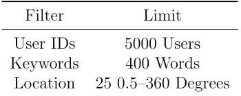
Twitter Streaming APIs. Of these, User Streams and Site Streams provide services oriented towards web applications that provide Twitter streams from the perspective of authenticated users. Although we considered establishing collections from the perspective of volunteer users, we ultimately dismissed this approach as impractical from a bureaucratic standpoint. Of the remaining options, the Twitter Firehose returns every status produced on Twitter and requires special access permissions. At over 500 million tweets per day [6], Firehose users need special infrastructure just to receive these data much less store them. Although we initially explored grants and relationships that would allow access to this API, we eventually decided that the engineering challenges surpassed the potential benefit to our project. This left the Public API, which provides the statuses/sample and statuses/filter endpoints. The Status Sample endpoint provides a straightforward “small random sample of all public statuses” [2]. The Status Filter returns public statuses that match one or more filters. These filters could be set over user IDs, keywords, or locations, under the constraints specified in Table 3.3. Due to these limitations, we chose to build a dataset from the Status Sample API. As detailed in Section 3.1.2, the Status Sample API provided a large volume of data to work with.
Streaming Endpoint Endpoint Type statuses/sample Public API
statuses/filter Public API user User Streams
site Site Streams statuses/firehose Firehose
Filter Limit User IDs 5000 Users Keywords 400 Words
Location 25 0.5–360 Degrees
Table 3.3: Filter Limits on statuses/filter
3.1.2 Collection
From the outset, our ambition was to collect a terabyte-scale dataset of Twitter messages in order to counteract the high dimensionality and sparsity of text data. To this end, our collection and storage platform was the bdserver Hadoop cluster consisting of one name node and 5 data nodes with a post-redundancy capacity of 26.9T. See Appendix A.1 for details on this machine and its configuration. This allowed us ample storage for not only the primary dataset but any files produced by subsequent data processing jobs. The MapReduce and YARN frameworks provided application-level tools for authoring distributed data processing jobs.
In order to facilitate collection, we authored the Java application twitter-fh to run for long periods of time on a server with access to a Hadoop file system. In addition to its collection capabilities, twitter-fh includes a publisher-subscriber architecture allowing it to be configured for logging, as well as multiple concurrent storage media and formats. Because Twitter aggressively cuts off multi-account stream subscriptions from the same machine, it was imperative that twitter-fh be powerful enough to handle multiple non-trivial stream subscriptions, particularly to the filter stream. This ex-tensible architecture allowed it to be easily modified when we needed to add additional behavior such as binned data storage and more complex stream subscriptions.
continuously, so it intermittently produced collections for the rest of 2014. This was less of a problem than one might think, as we still had ample data to work with from its initial collection runs. Rather than prioritizing 100% uptime, we chose to focus on data exploration of the initial output with the intention of executing a longer collection run when additional data was necessary. We observed a rough average of 20G per day in data volume, which we deemed sufficiently large for late-stage collection. In January 2015, full-time collection was resumed in earnest after fixing some of the technical issues with the collection program. Figure 3.1 illustrates the collection timeline for our data. Due to its relative continuity, most experiments were run considering only the 2015 dataset from January 6th to May 28th. These tweets were then separated and archived on the HDFS file system.
Aug Sep Oct Nov Dec Jan
2015 Feb Mar Apr May Jun 0
5 10 15 20 25 30
Daily GB Collected
GB
Figure 3.1: Daily Collection Volumes for 2014 through 2015
3.2
Processing Techniques
reference implementations. In general, these implementations were not designed for even gigabyte-scale datasets, and did not generalize well on terascale data. To reimplement many of them in a massively parallel context would be a separate thesis itself. On the other hand, YARN and MapReduce tools allowed us to easily collect simple statistics such as mean and standard deviation across our full dataset. In order to both leverage our large dataset and explore more sophisticated PGMs, we opted for a multi-stage data pipeline where YARN applications performed the dual tasks of statistics collection and dataset cleaning. These big data jobs produced much smaller, heavily filtered datasets suitable for the more sophisticated single-machine analysis algorithms. An added benefit of this approach was that with an overabundance of data, we had the luxury of discarding noisy or unhelpful sections of data that threatened to impede the performance of our topic models.
3.2.1 Big Data
For the initial data processing stages, we made heavy use of the Cascading data processing framework [1]. This open source framework provided a layer of abstraction on top of YARN and MapReduce, allowing us to develop data operations in terms of discrete “nodes,” which were then composed into a minimal number of MapReduce jobs. This paradigm allowed us to rapidly compose multiple MapReduce stages into one comprehensive data flow, and made large-scale data processing far more manageable and efficient. Via either aggregation, filtering or sampling, these data flows would produce cleaned datasets small enough for use in single-machine analysis.
Unlike earlier dual-role processing tasks, this task was created for the sole purpose of creating a cleaned corpus suitable for topic modeling. For the sake of brevity, we refer to this task as theTClean task, and its resulting dataset as theTClean dataset. Another, earlier dataset was theInfluenceFlow dataset, which performed aggregations and transformations to produce many derivative dataset features, while performing less aggressive filtering on the resulting corpus. As we will discuss in Chapter 4, the resulting size of this dataset eventually proved to be too unwieldly.
InfluenceFlow
The InfluenceFlow dataset was an initially simple tweet processing pipeline made with the intent of reformatting tweets for use with an L-LDA implementation, which grew over time to accomodate the various needs of different investigations. Although it performed many tasks, InfluenceFlow was organized around the principle of maximal data retention. Therefore, beyond very basic tweet cleaning stages the corpus was minimally filtered. Table 3.4 shows a number of statistics from different stages of the InfluenceFlow data processing task.
Metric Count
Raw Tweets 88,509,696 Cleaned Tweets 25,402,948 Hashtagged Tweets 4,691,545 Training Tweets 4,691,319
Testing Tweets 226
Unique Hashtags 1,012,176 Unique Users 9,913,571 User Interactions 19,143,165
TClean
The TClean dataset was produced at a late stage in this thesis, as the result of many earlier lessons learned. Earlier experiments had shown the significant scala-bility challenges of running new topic models on our dataset. Although large-scale implementations existed for common models such as LDA, these were highly specific and difficult to generalize to other candidate models such as LLDA, sLDA, and COLD. However, simply truncating the data to the first few million tweets would run the risk of producing a dataset where few similarities could be found across sparse language features. Instead, TClean was a dataset created to be a smaller, more manageable tweet corpus while still leveraging the increased sample size of the larger 2.5T collection.
A key insight was that LDA and its derivatives applied a statistical model to bag-of-word documents, and therefore, words which only occurred once contributed negligibly to the final model. Instead, stable models would extract co-occurence patterns between words and documents in the form of topics. A word could only be identified as a significant topic indicator if it ocurred relatively frequently in the corpus.
tweets containing “sufficiently typical” vocabulary. The full cleaning pipeline can be found in Table 3.5. Note that this process relies on two threshold values, t1 and t2, which filter out words and documents based on word frequency and document length.
Cleaning Step Description
Language Filter Remove any non-english tweets using metadata Deletion Notices Remove any tweets which are later deleted Lowercase Cast all tweet text to lowercase characters Character Filtering Remove punctuation and numerals
Tokenization Split tweets into words
Stopwords Remove topically neutral stopwords Stemming Stem words using the Porter Stemmer[28]
Word Frequency Filter Remove words which occur less than t1 = 200 times Document Length Filter Remove documents with a length less thant2 = 5
Table 3.5: TClean Cleaning Steps
To select appropriate word count threshold, we ran a tangential data flow which calculated word counts as well as the maximum threshold which would allow each document d ∈ D to remain in the corpus. We denote these value as sVw and sDd
respectively. We then calculated the number of occurrences for each value, denoted
fn? in Equations 3.1 and 3.2. This created an output dataset small enough to analyze on a traditional single-machine setup. Here a simple transformation gave us r? n
fnV ={w∈V |sVw =n}
(3.1)
fnD =|{d∈D|sd =n}| (3.2)
rnV =X i≥n
fiV (3.3)
rDn =X i≥n
fiD (3.4)
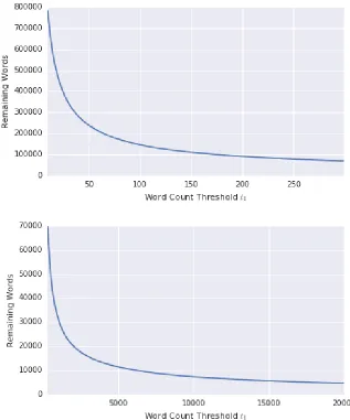
Upon investigation, we found that t1 had a much more pronounced effect on remaining word count rV than it did on remaining document count rD. Figure 3.2 depictsrV across varying scales oft
1, while Figure 3.3 depicts the similar relationship of rD and t
1. Both cases demonstrate a clear power law distribution, each function decreasing exponentially. We can also see that for threshold values as high as 20,000, the number of remaining documents is still over 70,000,000, while the number of remaining words has dropped to 5,000. This is consistent with our understanding of the corpus, since we can imagine that no matter how much we restrict the vocabulary, there will always be more tweets.
Figure 3.2: Effect of t1 Threshold on Remaining Word Count rVn on the domains
t1 ∈[15,300] and t1 ∈[3×102,2×104]
Cleaning Stage Count Input Tweets 703,558,103 Language Filter 172,432,743 Deletions 149,876,675 Deletion Filter 155,154,459 Threshold Fiter 88,443,396
3.2.2 Local Analysis
CHAPTER 4
HASHTAGS AND LLDA FOR POPULARITY
PREDICTION
Content on Twitter often encorporates special “hashtag” tokens, which are words prepended with the octothorpe “#” symbol (e.g., “#PorteOuverte” or “#YesAll-Women”). The web platform then converts these hashtags into hyperlinks to pages that display collected feeds of all tweets containing a particular hashtag. In this way, users can follow or participate in larger conversations by labeling their content with relevant hashtags. Hashtags can be interpreted as intuitive topic labels for content, curated by the entire microblogging community.
It has also been observed that hashtags play a dual role in social media. In addition to annotating content with similar topics, hashtags serve as a way for users to identify with a community. Yang et al. [36] demonstrated that this dual role can be used to effectively predict future adoption of hashtags by users based on their membership in a community. This work showed that hashtags symbolize not just topics but audiences around that topic [36]. Additionally, Suh et al. [33] have found evidence that hashtags “have a strong relationship with retweetability” [33]. With our hypothesis that retweetability could be predicted by a tweet’s topical content, we investigated the use of hashtags as features for retweet prediction.
formu-lating a predictive model that considered only hashtags for popularity prediction. If an effective model could be established, then it could be extended with topic models in order to draw the link between text content and hashtags. However, the first step was to confirm that hashtags were indeed effective features for popularity prediction, and to formulate a predictive model based on these isolated features.
4.1
Using Hashtags for Popularity Prediction
To model the relationship between hashtags and retweets, we formulated our inputs as a classic binary prediction problem. Given a tweet’s hashtags as input features (X), we endeavored to predict whether or not it would be a retweet (y) as a binary categorical variable. For the purposes of our initial study, we restricted the prediction problem to only those tweets that contained at least one hashtag in the InfluenceFlow dataset. As mentioned in Section 3.2.1, this constituted approximately 4.7 million tweets, or roughly 19% of the cleaned dataset.
Before we can discuss the input features for this model, we must first formalize how this problem is defined. First, for N documents, let D = [1, N] be a range of identifying numbers that can be bijected onto the set of documents. This allows for a convenient handle with which to refer to the documents, as well as an implied ordering for any matrix that contains information pertaining to the document. Similarly, for the vocabulary of M unique hashtags within the corpus, let H = [1, M] be a range of identifying numbers for these hashtags. In order to indicate whether a tweet uses a hashtag, let Idh# be the indicator for whether document d∈D uses hashtagh ∈H
of all tweets that use a particular hashtag, or all hashtags that a particular tweet uses. We refer to these with HD and D# as defined in Equations 4.3 and 4.4, respectively.
Idh# =
1 if d∈D uses h∈H
0 otherwise
(4.1)
IdR=
1 if d∈D is a retweet
0 otherwise
(4.2)
HdD =
n h ∈H
I
# dh = 1
o
(4.3)
Dh#=nd ∈D I
# dh = 1
o
(4.4)
With this formal structure in place, we sought to understand the probability that a message would be retweeted given its use of a hashtag. We denote this asp#h from Equation 4.5. Note that since hashtags are the only feature considered in this model, this probability is assumed to be invariant between documents as per Equation 4.6. Therefore, we do not index p# by any document d ∈ D. From here we estimate
p#h = PrIdR= 1|Idh# = 1 (4.5) (∀i, j ∈D)PrIiR= 1|Iih#= 1= PrIjR= 1|Ijh# = 1 (4.6)
ChR = X d∈D#h
IdR (4.7)
Ch6R =
D # h −C R h (4.8) ˆ
p#h = C R h D # h (4.9)
First, we note that ˆp#already represents a simple prediction model for whether a tweet will be a retweet. However, due to its formulation as a conditional probability, it is only suitable for tweets that use exactly one hashtag. For tweets that use more than one hashtag, we therefore take the mean of ˆp#h across all h ∈HdD to derive the metric ˆpA described in Equation 4.10. When we apply this to our test set from the InfluenceFlow corpus, which contains 206 tweets with one or more hashtags, we can measure its performance as a predictor. To measure classification performance, we use two common metrics: log loss (L) as defined in Equation 4.11, and area under the receiver operating characteristic curves (A or AUC) as defined in Equation 4.12.
While the former aims to demonstrate a reliable error for probability estimates of binary classifications, the latter showcases the performance of a model across all possible classification thresholds. The ideal score for a classifier would be L= 0 and A= 1. The performance of ˆpA under these metrics is shown in Table 4.1, along with
ˆ
pAd = 1 |HD
d |
X
h∈HD d
ˆ
p#h (4.10)
L(y,yˆ) = −1
N
N
X
n=1
[ynlog ˆyn+ (1−yn) log (1−yˆn)] (4.11)
A(y,yˆ) =
Z 1
0
TPRT(y,yˆ)FPR0T(y,yˆ)dT (4.12)
TPRT(y,yˆ) = True positive rate of ˆy using classification threshold T (4.13)
FPRT(y,yˆ) = False positive rate of ˆy using classification threshold T (4.14)
Metric Score
Log Loss (L) 1.620970 ROC AUC (A) 0.806827
Table 4.1: ˆpA Classification Performance
Having established ˆpA, we trained a logistic classification model using the
scikit-learn python library [13, 25]. Due to the large size of our dataset, it was impractical to train this model on each individual tweet. Instead, we relaxed our training algorithm to treat each unique hashtag as two weighted training points: one for positive retweet evidence and one for negative retweet evidence. Equations 4.15 through 4.20 express the training features of such a model. Note that for a given hashtag h∈H, the two observations X2h and X2h−1 take the same value of ˆp#h, while their yvalues are 1 and 0, respectively. Weighting is then used to represent that hashtag’s proportional usage in the dataset. This model formulation is equivalent to creating one observation of
ˆ
p#h, IdR
for every hashtag h in every document d, and then training our logistic classifier as normal. However, by using weights precomputed by a MapReduce task, we can drastically reduce the dimensionality of our dataset without any loss in accuracy.
X2h = ˆp #
h (4.15)
X2h−1 = ˆp#h (4.16)
y2h = 1 (4.17)
y2h−1 = 0 (4.18)
w2h =ChR (4.19)
w2h−1 =c
6
R
h (4.20)
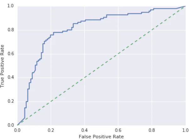
performance metrics for this classifier on the InfluenceFlow test set, while Figure 4.3 shows its receiver operating characteristic. Here it is evident that while the log loss has improved significantly, the AUC remains unchanged. This is consistent with our understanding of the logistic regression, since our classifier can be represented as a bijection between two monotonically increasing functions. As ROC analysis measures the performance of any possible classification threshold, every threshold on the original curve would be mapped to exactly one threshold point on the classifier’s predictions.
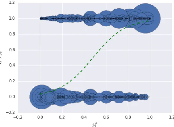
Figure 4.2: ˆpA Logistic Classifier Visualization
Metric Score
Log Loss (L) 0.576261 ROC AUC (A) 0.806827
Figure 4.3: ˆpA Logistic Classifier Receiver Operating Characteristic
We also investigated a second probability estimator ˆpBas defined in Equation 4.21. ˆ
pB is similar to ˆpA, but weights the mean of ˆp#h by the number of occurrences of hashtag h. Our aim was to create an estimator that was weighted by the evidence available for each input feature. However, as shown in Tables 4.3 and 4.4, it was categorically outperformed by ˆpA. We therefore gave it very little further attention. Rather than requiring readers to reread this chapter for comparisons, we have included a summary of scores in Table 4.5. Here we see that the logistic classifier on ˆpA is the strongest predictor among surveyed methods.
ˆ
pBd =
P
h∈HD d
ˆ
p#h D # h P
Metric Score Log Loss (L) 1.650664 ROC AUC (A) 0.783594
Table 4.3: ˆpB Clasification Performance
Metric Score
Log Loss (L) 0.624463 ROC AUC (A) 0.783594
Table 4.4: ˆpB Logistic Classifier Performance
X Method L A
Baseline yˆ=E[IR
d] 0.693637 0.500000 ˆ
pA yˆ=X 1.620970 0.806828
ˆ
pA Logistic Classifier 0.585102 0.806828 ˆ
pB yˆ=X 1.650664 0.783594
ˆ
pB Logistic Classifier 0.624463 0.783594
4.2
Identifying the Topic Spaces of Hashtags
After measuring the efficacy of hashtags as popularity predictors, we conducted a series of experiments investigating the possibility of mapping hashtags to topic vectors and vise versa. We hypothesized that by mapping content to topic-similar hashtags, we could make popularity predictions on untagged content that outperformed the baseline. We investigated LLDA as well as TF-IDF as mechanisms for performing this mapping, but ultimately found them both to be intractable for our purposes.
4.2.1 Labeled Latent Dirichlet Allocation
We have previously noted the role of hashtags as explicit topic labels for content. Labeled Latent Dirichlet Allocation (LLDA) is a topic model that accomodates ex-plicit topic labels, and has previously been successfully applied to recommendation tasks on microblogs [30, 31]. Using hashtags as topic labels, we investigated the use of LLDA in mapping hashtags to topic vectors. The advantage of this approach was that under the LLDA model, every hashtag maps to a single topic vector. Therefore, by estimating the topic distribution of an unlabeled document, its hashtag mapping would be made explicit by the model.
βk∼Dir(η) ∀k∈K (4.22)
Λd,k∼Bernoulli(Φ) ∀d∈D,∀k∈K (4.23)
L(ijd)=
1 if Λdi=j
0 otherwise
∀d ∈D (4.24)
α(d)=L(d)×α ∀d ∈D (4.25)
θd∼Dir α(d)
∀d ∈D (4.26)
zd,i ∼Mult (θd) ∀n∈Nd,∀d ∈D (4.27)
wd,n∼Mult (βzi) ∀n∈Nd,∀d ∈D (4.28)
Wd,n Zd,n
θd
α βk
η
Λd
Φ
∀n∈Nd
∀d∈D
∀k∈K
Figure 4.4: A Plate Notation Representation of LLDA [31]
exist one topic per unique hashtag, which would have an impact on the dimensionality of our estimated θ and β vectors. Due to the large scale of the training dataset, we expected this to be a large and long-running task.
Initial runs of the program encountered memory usage exceptions, indicating that the program was unable to scale to our full-sized dataset. All experiments were run on the infolab server (As discussed in Appendix A.2) in order to accomodate these large memory requirements. We therefore scaled back our approach, and ran JGibbLabeledLDA and the related JGibbLDA to explore its scalability properties. To control runtime, we created two truncated datasets of 5×10³ and 1×10⁵ tweets, respectively. Table 4.6 shows the runtimes and memory usage of running JGibbLDA and LGibbLabeledLDA on these datasets. We found that for datasets larger than 1×10⁵, runtimes became unmanageable and excessive memory usage often caused exceptions during execution. We attributed this result to the increased scale in-troduced by mapping hashtags to topics, and therefore having one topic for every unique hashtag. As shown in Table 4.6, the number of topics increases by two orders of magnitude. We can expect the peak memory usage to similarly expand to at least 400 GB, which is pushing the abilities of even our high-capacity infolab server. Furthermore, 1×10⁵ represents only a small fraction of our dataset, indicating that our LDA and LLDA implementations would be poorly equipped to train on the full InfluenceFlow corpus.
Records Algorithm # Topics Time Peak Memory Usage
5×10³ LDA 100 2m 16s 1.69 GB
5×10³ LLDA 1093 15m 17s 28.19 GB
1×10⁵ LDA 100 45m 36s 4.00 GB
1×10⁵ LLDA 11432 48h 49m 24s Unrecorded
Table 4.6: Run Times for LDA and LLDA tests
4.2.2 Token Correlation
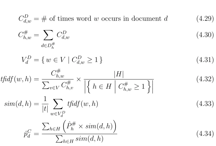
Cd,wD = # of times word woccurs in document d (4.29)
Ch,w# = X d∈Dh#
Cd,wD (4.30)
VdD ={w∈V |Cd,wD ≥1} (4.31)
tfidf(w, h) = C # h,w
P
v∈V C # h,v
× |H|
n
h∈H
C
# h,w ≥1
o
(4.32)
sim(d, h) = 1 |t|
X
w∈VD d
tfidf(w, h) (4.33)
ˆ
pCd =
P
h∈H
ˆ
Ph#×sim(d, h)
P
h∈Hsim(d, h)
(4.34)
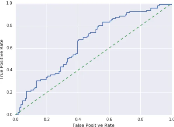
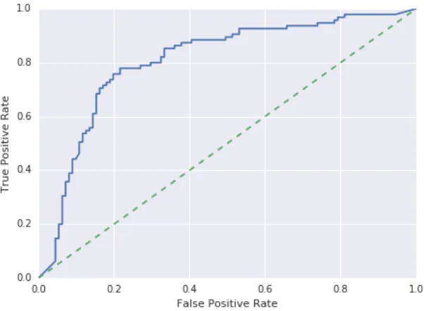
We then applied the measurement techniques from Section 4.2.1 to ˆpC. First we measured the performance of ˆpC as a predictor, and then that of the logistic classifier from Section 4.1 when ˆpC was applied as input. Tables 4.7 and 4.8 show the results of these measurements, while Figure 4.5 shows the corresponding ROC curve. Note that as in Section 4.1, the ROC curves are identical. Therefore, only one is included here. Furthermore, a prediction performance summary is again shown in Table 4.9.
Metric Score
Log Loss (L) 0.679541 ROC AUC (A) 0.648648
Table 4.7: ˆpC Clasification Performance
Metric Score
Log Loss (L) 0.765525 ROC AUC (A) 0.648648
Figure 4.5: ˆpC Logistic Classifier ROC Curve
X Method L A
Baseline yˆ=EIdR 0.693637 0.500000 ˆ
pA yˆ=X 1.620970 0.806828
ˆ
pA Logistic Classifier 0.585102 0.806828 ˆ
pB yˆ=X 1.650664 0.783594
ˆ
pB Logistic Classifier 0.624463 0.783594 ˆ
pC yˆ=X 0.679541 0.648648
ˆ
pC Logistic Classifier 0.765525 0.648648
In these tables, first observe that for ˆy = X, ˆpC drastically outperforms ˆpA and ˆ
pB. Although this was an interesting result, we could not derive any meaningful conclusions from it. As far as we can tell, it is little more than an interesting artifact of unfitted data. Much more legible were the results showing that L and A of the logistic classifier are significantly worse for ˆpC than that of the ˆpAor ˆpB. However, ˆpC still outperforms the baseline of ˆy= EIR
d
. From this, we concluded that hashtags can be used to predict the popularity of content, but that when available, using hashtags directly would result in better performance.
CHAPTER 5
DIRECT POPULARITY PREDICTION WITH SLDA
After concluding our investigation into the use of LLDA on popular hashtags, we shifted our focus to the potential of using another variant of LDA called Supervised Latent Dirichlet Allocation (sLDA) [23], which integrates characteristics of both topic modeling and a supervised learning task. We found this configuration to be an ideal candidate for a popularity prediction algorithm on topical features due to its integration of topic models with the supervised learning problem.
Supervised Latent Dirichlet Allocation is a statistical model introduced in col-laboration with the primary author on LDA, motivated by previous attempts by researchers to apply LDA to supervised learning tasks [23]. These applications address problems that can be broadly categorized as cases where text documents have an associated response variable that must be predicted. Many of these prior attempts used LDA-based topic models as input features for their regression methods, similar to our own attempts with LLDA. In contrast, the sLDA model integrates document response variables with the topic model itself. This allows for the estimation of topic vectors that are fitted not only to their content, but to the response variable itself.
applying a suitable distribution in the model. For example, if the response variable is categorical, a multinomial distribution could be used, while a real-valued response could be modeled with a gaussian distribution. However, both the original paper and our reference implementation described sLDA where the response is a normally distributed variable, so we will focus on that case here.
In such a case where the response variable y ∈R, sLDA takes the model param-eters described in Table 5.1. With these paramparam-eters established, each document and response is generated as follows:
1. For each document d∈D
(a) Draw topic distribution θd ∼Dir (α).
(b) For each word n∈N
i. Draw topic assignment zn|θ ∼Mult (θ).
ii. Draw word from topic wn|zn, β1:K ∼Mult (βzn).
(c) Draw response variable y|z1:N, η, σ2 ∼N η>z, σ¯ 2
.
¯
z = N
X
n=1
zn (5.1)
In this process, ¯z is the weighted average between drawn topics, as defined in Equation 5.1. This generative process is illustrated in plate notation by Figure 5.1, providing a convenient graphical representation.
Parameter Description
K Number of topics.
V Number of unique words.
α The document-topic dirichlet parameter
β1:K The topic vectors, each a βk being a V-dimensional multinomial distribution. In our reference implementation, these are themselves estimated from a dirichlet prior in the same fashion as an LDA model.
η A vector of response means whereηk is the mean response for topick.
σ A vector of response deviations whereσk is the standard deviation for topic k.
Table 5.1: Model Parameters for sLDA
Wd,n Zd,n
θd α
Yd η, σ2 βk
∀n∈N
∀d∈D
∀k∈K
the efficacy of this approach. Our experiments with sLDA centered around running it on our TClean dataset, with a document’s retweet status as its signal variable.
Rather than reimplementing sLDA for our experiments, we sought to use a ref-erence implementation to save time and effort. Although we considered the original implementation released by Mcauliffe and Blei [23], we ultimately used the R imple-mentation found in the “lda” R package on CRAN for its speed and usability. Whereas the original implementation performs its estimation via variational inference, the R sLDA implementation instead uses collapsed Gibbs sampling.
After our experiences with LLDA, we deemed the challenge of running sLDA on the full-scale dataset to be out of scope of our project, and instead invested our time on creating the newTCleandataset described in Section 3.2.1. It is important to note that in order to achieve data reduction, TClean aggressively filters content from the original dataset down to content with a “representative” vocabulary, meaning that any results we arrive at are for a particular kind of tweet. Specifically, the results of this study describe the performance of sLDA on tweets that satisfy the vocabulary frequency constraints described in Section 3.2.1, which corresponds to a tweet using a sufficient “median vocabulary” of tokens that occur more frequently than most within the corpus.
Xdw = # of occurences ofw in d (5.2)
yd =
1 if d is a retweet
0 otherwise
(5.3)
In these experiments, we aimed to answer the following questions:
1. What sLDA parameters led to the best retweet predictions?
2. How did these predictions compare to our hashtag-based model in Chapter 4?
3. Were these predictions sufficiently accurate to indicate a correlation between tweet topics and retweets?
5.1
Parameter Selection for SLDA
For the purposes of our experiment, our ultimate goal was a configuration of sLDA that produced predictions as accurately as possible. However, our reference imple-mentation took multiple tuning parameters, some of which had large impacts on the ultimate running time of the process. Other parameters had little impact on running time, but would need to be adjusted to maximize performance. We first investigated parameters with high impacts on time performance to see if we could observe trends in speed and performance. From there, we used our results to run longer sLDA runs using the knowledge we had gained from shorter runs.
time, in addition to the dimensionality of the dataset itself. Whileeandmmodulated the number of gibbs sampling sweeps and the number of expectation maximization iterations, respectively, k controlled the number of latent topics that would be used in the model. These were the variables we chose to focus on in our preliminary runs, so that we could gather performance data that could later inform more expensive computations.
Parameter Description
K, α, η, β, σ Model parameters. See Table 5.1.
e The number of Gibbs sampling sweeps to make over the entire corpus for each iteration of EM.
m The number of EM iterations to make.
Table 5.2: Estimation Parameters for sLDA
5.1.1 Sweep 1E5–1
L=−1
N X
i=1
yilog ( ˆyi) + (1−yi) log (1−yˆi) (5.4)
ˆ
yd= Predicted yi given Xi (5.5)
First, we truncated the TClean dataset down to its first 105 tweets, denoting this new dataset TClean5. This allowed us to run sLDA estimations in a shorter amount of time, which seemed reasonable as the original authors used datasets with even fewer documents in their original paper [23]. After truncation, TClean5 was split into randomly sampled training and testing sets, at a ratio of 80% training records to 20% testing. Training records were further segmented into 3 equally sized validation folds (F = 3), again using random sampling.
The sweep itself was then performed across the range of values described in Table 5.3. For each iteration in the sweep, a sLDA model would be cross-validated over the validation folds using parameters from the range in Table 5.3, as well as the static parameters described in Table 5.4. We measured both the time elapsed while estimating the model, as well as the log-loss prediction performance of the estimated model on the held-out validation fold. With 3 validation folds, this allowed us to take the mean and standard deviation of each parameter set, in order to confirm that our measurements were representative for a given parameter set. Table 5.5 provides a summary of these measurements, as well as the derived values used in later analysis. All runs were performed on the Sweet Chedda machine discussed in Appendix A.3.
Parameter Start End Step Size
e 10 80 10
m 2 10 2
k 10 40 10
Parameter Value
F 3
α 1/K
β 1/V
η Retweet signal mean in training set
σ2 Retweet signal variance in training set Table 5.4: Static Parameters for sLDA Sweep 1E5–1
Measure Description
Lfemk Log loss for sLDA model on training fold f with parameters e, m, and
k. See Equation 5.4. ˆ
Lemk Mean log loss for sLDA model with parameters e, m, and k. See Equation 5.6.
σL
emk Standard deviation of log loss for sLDA model on training fold f with parameters e, m, and k. See Equation 5.7.
ErrLemk Estimated 3σerror of ˆLemkas a percentage of its value. See Equation 5.8.
tfemk Elapsed seconds for training sLDA model on training fold f with pa-rameters e, m, and k.
ˆ
temk Mean elapsed seconds for sLDA model with parameterse,m, andk. See Equation 5.6.
σt
emk Standard deviation of elapsed seconds for sLDA model on training fold
f with parameters e, m, and k. See Equation 5.7.
Errtemk Estimated 3σerror of ˆtemk as a percentage of its value. See Equation 5.8.
Table 5.5: Measurements from sLDA Sweep 1E5–1
ˆ
Lemk = 1
F X
f∈F
Lfemk (5.6)
σemkv =
s
1
F X
f∈F
vemkf −vˆemk
2
(5.7)
Errvemk = 100× 3σ v emk ˆ
vemk
The measured effects ofe,m, andkon ˆLandtare summarized in Figure 5.2, which illustrates ˆLemkand ˆtemkfor all permutations ofe,m, andk. Figure 5.3 illustrates the corresponding values of ErrLemk and Errtemk. From these figures, we drew the following key observations:
1. Almost all Erremk error bars fell below 3% of their values, indicating that there would likely be little variation between estimation runs in relation to measured values. Outliers were primarily for low values of ˆtemk.
2. Despite this, the magnitude of 3σemk is often greater than the differences be-tween ˆLemkand ˆtemkfor different values of input parameters. This would suggest that it is not uncommon to have observations where one set of parameters outperforms another, even when its average performance would be worse. In other words, due to the variations between folds, the advantage of one parameter set over another is only measurable over multiple folds.
3. For k = 10, ˆLemk indicated little visual correlation with any values of e or m. However, as k increased to higher values, ˆLemk displayed a negative correlation with both e and m values, particularly for the higher values of k = 30 and
k = 40.
4. ˆLemk also seemed to take lower values for higherk.
increased time required to estimate the corresponding model. Therefore, we aimed to discover the combinations of e, m, and k that would yield optimal prediction performance for a given timeframe.
Before exploring what such an optimal combination would look like, we first took some time to establish the relationship between e, m, k, and ˆtemk. If we were to vary any one of these constants, holding the others fixed, we would expect the time complexity to increase linearly. Therefore, we hypothesized that ˆtemk≈c×e×m×k, for somec∈R≥0. However, since this was a minor corrolary to our study, we chose to
validate this empirically rather than performing a complexity analysis. To this end, we derived the dimensionality measure Dimemkdefined in Equation 5.9 and performed a linear regression between Dimemk and ˆtemk, in addition to measuring the Pearson correlation coefficient. The results are listed in Table 5.6, as well as displayed visually in Figure 5.5. With a correlation coefficient of r ≈ 0.999155, we were confident in the linear relationship between Dimemk and ˆtemk. This would be useful later, when we wanted to run sLDA estimations for a particular duration.
Dimemk =e×m×k (5.9)
Parameter Value Slope 0.008330 Intercept 1.448136 RValue 0.999155 PValue 0.000000 StdErr 0.000016
Table 5.6: Sweep 1E5–1 Dimensionality vs Timing Regression Results
sLDA estimation time, we then turned to examining the more ambiguous relationship between these variables and ˆLemk. Figure 5.6 provides an entry point for this relation-ship, suggesting the trend that as we spend more time estimating our model, the log loss of its predictions will decrease. Seeking to investigate this relationship further, Figure 5.7 displays the same scatter plot with logistic regression lines overlayed for different values ofe,m, andk. Although this is far from a conclusive solution, we can observe that while regression lines foreandm are somewhat disordered, those for the
k plot show a clear anticorrelation between k and ˆLemk. Even for measurements of roughly the same duration, a higherk seems to correlate to better performance in the model. We found this relationship to be less qualitatively obvious in our explorations of e and m. Figure 5.8 deconstructs Figure 5.7 further by separating measurements by theirkvalue. Here we can see that trendlines forkdecrease in slope ask increases. This would suggest that not only is a higher k better, but it has a higher potential for performance gains as the model runs longer.
It is important to note that the previous observations are all qualitative in nature. Although these trends are highly suggestive, they do not alone indicate any sort of optimal combination of e, m, and k, nor the tradeoffs associated with sacrificing one for another. After numerous attempts, we still struggled to tease out this deeper relationship between ˆLemk and e, m, and k. We eventually decided to perform a second sweep, using what we knew about the time complexity of our problem to run another sweep across e,m, and k that held time constant.
5.1.2 Sweep 1E5–2
of sLDA models parameterized on e, m, and k. However, Sweep 1E5–2 used our knowledge of ˆtemk from Section 5.1.1 to select values for e, m, and k, which had the same runtime by holding Dimemkconstant. Having confirmed the correlation between Dimemkand ˆLemk, we hoped that by isolating it from the equation we could shed some light on the interplay between e,m, and k in the same time context.
In this sweep, we chose to select Dimemk approximately corresponding to runtimes of ˆtemk ∈ {180,300,420} (3–7m). This led to Dimemk taking the values in Table 5.7, which also describes the sweep ranges for m and k. The e variable was fixed by the other time sensitive parameters, as described in Equation 5.10 (in order to satisfy the relationship defined in Equation 5.9). Other parameters were identical to those used in Sweep 1E5–1, as described in Table 5.4.
Parameter Start End Step Size Dimemk 21000 49000 14000
m 2 10 2
K 50 250 50
Table 5.7: Ranges for sLDA Sweep 1E5–2
e = Dimemk
mk (5.10)
the obvious anticorrelation between ˆLemk and k. However, the other anticorrelations with e, m, and Dimemk from Sweep 1E5–1 are all less apparent. This could perhaps be explained by the large difference in scale between k and the other parameters.
Before investigating further, we confirmed that our observation from Section 5.1.1, that ˆLemk and Dimemk are anticorrelated, still held for Sweep 1E5-2. Figure 5.12 illustrates that this still appears to be the case. As dimensionality of sLDA increases, the mean log loss of its predictions can be observed to steadily decrease. We quantify this relationship in Table 5.8 by calculating Pearson’srcorrelation coefficient between Dimemk and ˆLemk. The resulting value of ρDim,Lˆ = −0.178 tells us that the anticor-relation is noisy, but measurable. Although it is difficult to accurately measure the significance of this correlation, it provides a baseline of comparison between Dimemk,
m, and k.
X ρX,Lˆ
m -0.021126
k -0.754449
Dimemk -0.178567
Table 5.8: Pearson’sr Correlations of ˆLemk
Figure 5.12: Dimensionality vs Log Loss for Sweep 1E5–2
Figure 5.14: k vs Log Loss for Sweep 1E5–2
These patterns were consistent with our own understanding of the sLDA model, and the difference betweeneorm andk. Wherease andm are variables that control the number of iterations given for the model to converge, k increases the model’s available degrees of freedom. Therefore, after e and m are set to values sufficiently large enough for the model to converge, we would expect very little improvement in performance by increasing them further. On the other hand, increasing k allows a fitted model to capture additional information. The lack of any discernible trend between m and ˆLemk suggests that for the values considered in Sweep 1E5–2, the model has entirely converged.
5.1.3 Sweep 1E5–3
continued to adjusteaccording to Equation 5.10 as in Sweep 1E5–2, as well as 3-fold cross validation. It is important to note that in this sweep we still hold dimensionality constant, meaning that as we increase k, we have fewer iterations available in e to converge on a solution.
Parameter Value Dimemk 35,000
m 2
Table 5.9: Static Parameters for sLDA Sweep 1E5–3
Parameter Start End Step Size
K 50 1250 50
Table 5.10: Ranges for sLDA Sweep 1E5–3
From the results in Sweep 1E5–3, we found that as k increased, its benefits were eventually reversed. Figure 5.15 depicts the mean Log Loss of our sLDA model as we vary k, along with its associated error bars. We can see that the model exhibits optimal mean performance at k = 600, which corresponds to e = 29. However, it is also notable that these results are fairly noisy, and given the various local minima surrounding k = 600, it is possible that the true minimizing value for k might be as low as 350 or as high as 750 if we were to increase our sample size. Nonetheless, this operational range gives us enough information to estimate roughly optimal parameters for larger dataset sizes.
values ofk did a poorer job of capturing information, contrary to our assumptions of the model. However, investigating this distinction was beyond the scope of our goals. We instead concluded that we should use k = 600 when training our final model for use on the test set, and moved on to measuring the performance of sLDA on the held-out testing set.
5.2
SLDA Performance Analysis
Having determined good estimates for optimal parameters for sLDA, we moved on to testing it against the held-out test set, and comparing its performance to a number of other benchmarks. We proceeded to train our sLDA model on the full TClean training set, alongside our reference models, and then test them on the corresponding held-out test set. We found that although sLDA succeeded at predicting retweets to some degree, it was outperformed by another widely available model.
In addition to sLDA, we trained the two Naive Bayes models shown in Table 5.11, as well as an ensemble classifier to test the possibility of combining the output of sLDA with that of our best performing classifier. For the sLDA model, we chose tuning parameters of e = 200, m = 3, and k = 600. Here we used the optimal k
ascertained in Section 5.1, but chose to increase oure andm values in order to avoid the accuracy tradeoff discussed at the end of the same section. We also evaluated a simple baseline, where every predictionywas equal to the retweet ratio in the training set.
Model X Parameters
sLDA Token Counts e = 200, m= 3, k = 600
Multinomial Naive Bayes Token TFIDF Bernoulli Naive Bayes Hashtag Count
Ensemble SGD Logistic Classifier sLDA & Naive Bayes loss = Log-Loss
Table 5.11: Tested Predictive Models
same methods as the other models. Table 5.12 shows a performance summary of the evaluated models, while Figures 5.16 through 5.19 show the corresponding ROC curves. SLDA performed better than the simple baseline and the hashtag-based Bernoulli Bayes, but was outperformed by the text-based Multinomial Naive-Bayes. We then took the output of sLDA and Multinomial Naive Bayes and used them as inputs to an Ensemble SGD Logistic Classifier to test the hypothesis that by combining both approaches, we could outperform Multinomial Naive Bayes alone. However, we found that the ensemble classifier had significantly worse log-loss than Multinomial Naive Bayes, indicating that the noise introduced by considering both outputs outweighed the gain in information.
Model L A
sLDA 0.611700 0.683622
Simple Baseline 0.665830 0.500000
Multinomial Naive Bayes 0.563959 0.741970 Bernoulli Naive Bayes 0.628331 0.607087 Ensemble SGD Logistic Classifier 0.595622 0.704890
Table 5.12: Summary of Predictor Performance
Figure 5.16: sLDA Classification ROC Curve
Figure 5.18: Bernoulli Naive Bayes Classification ROC Curve
![Figure 3.3: Effect of t1 Threshold on Remaining Document Count rDn on thedomains t1 ∈ [15, 300], t1 ∈ [3 × 10², 2 × 10⁴], and t1 ≥ 2 × 104](https://thumb-us.123doks.com/thumbv2/123dok_us/8921278.1841712/34.612.166.469.113.699/figure-eect-threshold-remaining-document-count-rdn-thedomains.webp)
![Figure 4.4: A Plate Notation Representation of LLDA [31]](https://thumb-us.123doks.com/thumbv2/123dok_us/8921278.1841712/46.612.179.544.82.508/figure-a-plate-notation-representation-of-llda.webp)