DEMOGRAPHIC RESEARCH
A peer-reviewed, open-access journal of population sciences
DEMOGRAPHIC RESEARCH
VOLUME 36, ARTICLE 26, PAGES 745–758
PUBLISHED 14 MARCH 2017
http://www.demographic-research.org/Volumes/Vol36/26/
DOI: 10.4054/DemRes.2017.36.26
Descriptive Finding
Generalised count distributions for modelling
parity
Bilal Barakat
c
2017 Bilal Barakat.
1 Introduction 746
2 Generalised count distributions 748
2.1 The Conway-Maxwell-Poisson distribution (COM-Poisson) 748
2.2 The gamma count distribution 749
2.3 General comments 749
2.4 Gamma count as a Swiss army knife 750
3 Empirical analysis 752
3.1 Completed cohort parity from the Human Fertility Database 752
3.2 Zero inflation 753
3.3 Fits to empirical parity distributions 755
4 Conclusion 756
Generalised count distributions for modelling parity
Bilal Barakat1
Abstract
BACKGROUND
Parametric count distributions customarily used in demography – the Poisson and neg-ative binomial models – do not offer satisfactory descriptions of empirical distributions of completed cohort parity. One reason is that they cannot model variance-to-mean ra-tios below unity, i.e., underdispersion, which is typical of low-fertility parity distributions. Statisticians have recently revived two generalised count distributions that can model both over- and underdispersion, but they have not attracted demographers’ attention to date.
OBJECTIVE
The objective of this paper is to assess the utility of these alternative general count distri-butions, namely the Conway-Maxwell-Poisson and gamma count models, for the model-ing of distributions of completed parity.
METHODS
Simulations and maximum-likelihood estimation are used to assess their fit to empirical data from the Human Fertility Database (HFD).
RESULTS
The results show that the generalised count distributions offer a dramatically improved fit compared to customary Poisson and negative binomial models in the presence of under-dispersion, without performance loss in the case of equidispersion or overdispersion.
CONCLUSIONS
This gain in accuracy suggests generalised count distributions should be used as a matter of course in studies of fertility that examine completed parity as an outcome.
CONTRIBUTION
This note performs a transfer of the state of the art in count data modelling and regression in the more technical statistical literature to the field of demography, allowing demogra-phers to benefit from more accurate estimation in fertility research.
1. Introduction
The number of live births a woman experiences, her parity, is an integer count. The sta-tistical analysis of parities therefore requires the use of discrete count distributions. Fully nonparametric approaches are an alternative in some, but by no means all, applications and suffer serious disadvantages of their own, notably a lack of analytic parsimony. Un-fortunately, the choice between parametric count distribution has until recently effectively been limited to the Poisson distribution and the negative binomial distribution, including in demographic analysis (e.g., Parrado and Morgan 2008; Nis´en et al. 2014).
It is well known that the variance-to-mean ratio of a Poisson distribution, its disper-sion, equals one by construction. Accordingly, Poisson distributions fit poorly to empir-ical distributions whose dispersion differs considerably from unity. In applied statistics generally, attention has largely focused on the need to account for overdispersion, that is, dispersion considerably larger than one. This is unsurprising, given that mixtures of Pois-son distributions are always overdispersed and heterogeneity is one of the most common ways in which we expect reality to diverge from simple statistical models. Indeed, both the negative binomial distribution and the ‘zero-inflated’ Poisson, where a certain share of structural-zero outcomes are assumed, can be mathematically interpreted as special cases of Poisson mixtures, and, like the regular Poisson distribution, they are structurally unable to model underdispersion.
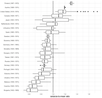
The need for alternative modeling options in the context of human birth parities arises from the fact that in low-fertility settings underdispersion is actually the norm, in other words: parity distributions whose mean considerably exceeds their variances. Figure 1 demonstrates this using data from the Human Fertility Database (HFD).
Statistically speaking, underdispersion could arise as a consequence of: a) a positive interpersonal correlation in terms of the child count, b) mechanisms that diminish the occurrance of ‘runaway’ parity, where some women tend towards extremely high birth counts while others are ‘stuck’ at low levels, namely a parity progression rate that is negatively related to the parity already achieved, or c) a parity progression rate that is positively correlated with the waiting time since the last birth.
Figure 1: Statistical dispersion (variance-to-mean ratio) in completed cohort parity distributions of the HFD, by country, across birth cohorts (in parentheses)
Bulgaria (1932−1969) Czechia (1935−1974) Belarus (1949−1974) Ukraine (1944−1973) Estonia (1944−1974) Portugal (1944−1972) Norway (1952−1974) Russia (1944−1974) Taiwan (1961−1974) Hungary (1937−1974) Slovakia (1935−1969) Germany (1941−1950) Slovenia (1968−1974) Sweden (1955−1974) Spain (1960−1974) Lithuania (1955−1974) Netherlands (1935−1972) Japan (1953−1974) Canada (1929−1971) United States (1918−1974) Austria (1969−1974) Finland (1967−1972)
0.6 0.8 1.0 1.2 1.4 1.6
variance-to-mean ratio
2. Generalised count distributions
2.1 The Conway-Maxwell-Poisson distribution (COM-Poisson)
This distribution was originally proposed by Conway and Maxwell (1962) and more re-cently revived by Shmueli et al. (2005). It generalises the standard Poisson distribution by allowing the probabilities to decay more rapidly or more slowly as the distance from the mean increases. As such, it formalises mechanism b) above. Formally, its probability function takes the form:
P(Y =n) = λ
n
(n!)ν 1
Z(λ,ν),
for n = 0, 1, 2,. . ., where the normalising constant is Z(λ,ν) = P∞ i=0,
λi
(i!)ν and the
parameters must satisfy the constraints λ > 0,ν ≥ 0. Parameters λand ν may be
interpreted as representing the rate and dispersion of the distribution in the general sense that for fixedν the mean of the distribution increases withλ, and that for fixed λ, the
distribution becomes more spread out for decreasingν. Unfortunately, no closed-form
expression exists to relate these parameters to the distribution’s moments directly. Our intuitive interpretation of the parameters must therefore rest on the fact that the ratios of successive probabilities can be expressed simply as:
P(Y =n−1)
P(Y =n) =
nν
λ .
This means thatλdetermines the overall relationship between the probabilities at
succes-sive parities whileν determines how these relationships change with increasing parity.
Forν = 1this reduces to the regular Poisson case, whileν < 1andν > 1 result in overdispersion or underdispersion, respectively. In the HFD data analysed here, the esti-mated values ofλor range from 1.4 to 27.8, andνranges from 0.8 to 3.8. This excludes 17 country-cohort dyads (out of 579) with extremely low or high variance-to-mean ratios for which the estimates suffered from convergence problems.
2.2 The gamma count distribution
Specifically, the gamma count model takes the following form:
P(Y =n) =G(αn,βT)−G(α(n+ 1),βT) (1) forn= 0, 1, 2,. . ., whereG(αn,βT)is the regularised lower incomplete gamma func-tion
G(αn,βT) = 1 Γ(nα)
Z βT
0
unα−1exp−u du
andT is the scale of the overall exposure period. We haveα,β ∈R+andG(0,βT)≡
1 by assumption. In our setting T = 1 may be assumed without loss of generality.
Asymptotically,αis the dispersion factor, αβ is the mean waiting time between births,
andβαapproaches mean parity. Note, however, that these asymptotic approximations can
be poor in the parameter range of interest for fertility applications and should not be relied
on. Forα= 1the model reduces to the special case of Poisson counts, andα <1and
α > 1result in overdispersion or underdispersion. In the HFD data analysed here, the estimated values ofαrange from 0.8 to 4.5, andβranges from 1.4 to 10.8.
2.3 General comments
A well-known property of the standard Poisson model is that the number of events per unit of exposure is a sufficient statistic for the mean. In practice this is frequently exploited to allow for the aggregation of data without loss of information: For any given values of possible covariates, only the total amount of exposure and total number of events needs to be recorded. It is important to note that neither the COM-Poisson nor the gamma count model allow for this operational shortcut. Because the hazard is a nonconstant function of the waiting time or parity already attained, the way the eventless episodes are distributed between individuals does matter.
Existing implementations of the COM-Poisson model are available in the
compoisson,CompGLM, andComPoissonRegpackages forR, for instance, as well
as forSAS(in theCOUNTREGprocedure) andMATLAB, but not – to the best of my
knowl-edge – forSTATA. The gamma count model does not currently appear to be available off
the shelf on any platform, but its definition (Eq. 1) is straightforward to implement in terms of the gamma function. This approach was followed here. The code underlying the present analysis is available as anRpackage alongside this article and was executed by
2.4 Gamma count as a Swiss army knife
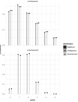
Fortunately, what initially appears as a potentially confusing proliferation of options for modelling count data ultimately leads to a simplification. Figure 2 shows both the COM-Poisson and gamma count models fitted to an overdispersed target drawn from a negative binomial distribution and the gamma count model fitted to an underdispersed target drawn from a COM-Poisson distribution. This illustrates two points: Firstly, it shows that the availability of fully generalised count distributions makes the negative binomial model practically redundant for human parity modelling, because it can be well approximated by the COM-Poisson or gamma count models of overdispersion within the relevant range of mean parity and dispersion. Secondly, it shows that their unique ability to model underdispersion sets the latter two distributions apart from other count models, but not from each other, because they can mimic each other very closely. This was tested for this study across the entire parameter range of interest in fertility applications. As a matter of fact, the case displayed in Figure 2 displays the maximal discrepancy found, with the typical error being an order of magnitude smaller than the one shown here.
Figure 2: Simulated parity distributions resulting from maximum-likelihood fits of: COM-Poisson and gamma count models to an overdispersed target distribution sampled from a negative
binomial distribution (top panel), and a gamma count model to an underdispersed target sampled from a COM-Poisson distribution (bottom panel)
underdispersed overdispersed
0 1 2 3 4 5
0.0 0.1 0.2
0.0 0.1 0.2 0.3 0.4
parity
probability
distribution
NegBinom
COMpoisson
GammaCount
waiting times, either the COM-Poisson model or gamma count model may be more ap-propriate. Similarly, for regression analysis the choice of model is dictated by whether the dependent variable is mean waiting time or mean birth count directly. Thirdly, the purpose of modelling may be decisive, because the two distributions differ in their prac-tical properties. While the statisprac-tical properties of the COM-Poisson model have been investigated more fully (Sellers and Shmueli 2010) and asymptotic significance tests are available, the gamma count model has the advantage that it appears to be vastly more efficient computationally, by one or two orders of magnitude. This is no doubt due to the fact that the underlying gamma function benefits from being a common mathematical function for which highly optimised algorithms are standard. The gamma count model may therefore be preferable for simulation and inferential approaches involving frequent (re)sampling from the distribution, namely both bootstrapping and Bayesian inference.
So while there is a role for the COM-Poisson distribution for certain applications, a case can be made for the gamma count distribution as a general-purpose default for modeling both over- and underdispersed distributions of human birth parities.
3. Empirical analysis
3.1 Completed cohort parity from the Human Fertility Database
The Human Fertility Database, at least with respect to time series of parity completed by age 40, is focused on industrialised high-income countries.
3.2 Zero inflation
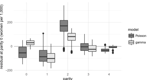
Figure 3 displays the average absolute residual by parity. The pattern of these residuals for the Poisson model is dominated by the relatively large share of women with two children. This means that both parity 0 and positive parities contribute to the observed underdispersion.
While the gamma model evidently represents a significant improvement over the Poisson (and equivalent NegBinom) fit in the underdispersed case, the question whether its fit is already good enough in absolute terms needs to be reviewed critically depending on the application. In particular, examples can be found across a wide range of parity pat-terns where the empirical pattern is not modelled satisfactorily, including some or most cohorts in Canada, Hungary, or Japan, among others (for assessing the fits to individual country-cohort-specific parity distributions, ‘rootograms’ [Kleiber and Zeileis 2016] can be generated within theRpackage accompanying this article). This suggests that the way these empirical parity distributions differ from the Poisson idealisation is not limited to the presence of underdispersion. Crucially, as can be seen in Figure 3, the residual devi-ation remaining after allowing for underdispersion is systematic, in that a large residual remains at parity 1 specifically. Nonetheless, as shown in the following, while the simple gamma model by itself cannot match this pattern, it does pave the way for significantly reducing the residual in a way the Poisson model does not. The key lies with parity 0, rather than parity 1, however.
Figure 3: Absolute residuals (observed – fitted) by parity of maximum-likelihood fits of different models to empirical HFD distributions of completed cohort parity, across countries and cohorts, in terms of women per 1,000
−200 0 200
0 1 2 3 4
parity
residual at par
ity 0 (w
omen per 1,000) model
Poisson
gamma
Note: Thick horizontal line: median across cohorts; box: inter-quartile range (IQR); whiskers: observations within 1.5 times IQR; points: outliers.
To gain some insight into the relationship between zero inflation on the one hand and the regular Poisson and gamma count distributions on the other (the negative binomial and COM-Poisson models add no information since their fits are each practically identical to the one shown), focus on parity 0 in Figure 3. It is evident that, in general, the regular Poisson model predicts too many zeroes rather than too few. This is unsurprising; we know the vast majority of HFD parity distributions to be underdispersed. By observing that a probability point mass at zero can be interpreted as a Poisson distribution with mean and variance zero, it becomes clear that the zero-inflated Poisson model is actually a special case of a mixture of Poisson distributions. Accordingly, it always results in overdispersion. An underdispersed distribution is therefore unlikely to exhibit excess zeroes relative to a regular Poisson distribution.
avail-able to the Poisson model (or indeed, the negative binomial model), which is already overestimating the proportion at parity 0.
3.3 Fits to empirical parity distributions
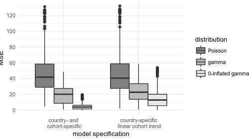
With this in mind, Figure 4 compares the fits of the regular Poisson, gamma count,and
zero-inflated gamma count models to the empirical HFD completed-cohort birth parity distributions, in terms of mean squared error based on the original scale of women per 1,000. To simplify the presentation, the redundant negative binomial and COM-Poisson fits are omitted again. The former is redundant because most of the observed distributions are underdispersed, and so the negative binomial would reduce to the Poisson case. The latter is redundant because we already established that the COM-Poisson and gamma count distributions closely mimic each other in the relevant parameter range and therefore perform approximately equally well in fitting the empirical data.
Figure 4: Mean squared error (MSE) of maximum-likelihood fits of different models to empirical HFD distributions of completed cohort parity, across countries and cohorts, in terms of women per 1,000
0 20 40 60 80 100 120
country- and cohort-specific
country-specific linear cohort trend
model specification
MSE
distribution
Poisson
gamma
0-inflated gamma
Note: Thick horizontal line: median across cohorts; box: inter-quartile range (IQR); whiskers: observations within 1.5 times IQR; points: outliers.
models. However, even the three-parameter zero-inflated gamma count distribution can-not be said to be overfitted. Technically the fit here is to 11 data points for each distribu-tion, namely parities 0 through 10, but even restricting attention to those with meaningful frequencies – 0 to 5, say – still leaves the data with six degrees of freedom. So even the most complex of the three models is still parsimonious, with the additional param-eters all enjoying meaningful substantive interpretations and achieving a fit as close to perfect as one can hope for in modelling natural phenomena: The mean squared error of the zero-inflated gamma count model is less than nine in the vast majority of cases, and typically closer to four, which means its predicted values generally differ from the ob-served values by only two or three women per 1,000. Moreover, the right set of box plots demonstrates that the great improvement in fit over the Poisson distribution is certainly not due to approximating a saturated model: This specification assumes linear (over co-horts) country-specific trends in each parameter, and therefore uses two (Poisson), four (gamma count), or six (zero-inflated gamma count) parameters, respectively, to fit all par-ities 0 through 10 for between 6 (Austria, Finland) and 57 (USA) cohorts at once. While merely illustrative, this specification is close to applications in real-life research in terms of its general structure.
4. Conclusion
References
Conway, R.W. and Maxwell, W.L. (1962). A queuing model with state dependent service rates.Journal of Industrial Engineering12(2): 132–136.
Human Fertility Database (HFD). Max Planck Institute for Demographic Research
(Germany) and Vienna Institute of Demography (Austria). Available at
www.humanfertility.org (data downloaded on [2016-10-21]).
Kleiber, C. and Zeileis, A. (2016). Visualizing count data regressions using rootograms.
The American Statistician70(3): 296–303. doi:10.1080/00031305.2016.1173590.
Nis´en, J., Myrskyla¨a, M., Silventoinen, K., and Martikainen, P. (2014). Effect of
family background on the educational gradient in lifetime fertility of
Finnish women born 1940–50. Population Studies 68(3): 321–337.
doi:10.1080/00324728.2014.913807.
Parrado, E.A. and Morgan, S.P. (2008). Intergenerational fertility among hispanic women:
New evidence of immigrant assimilation.Demography45(3): 651–671.
R Core Team (2016).R: A language and environment for statistical computing. Vienna:
R Foundation for Statistical Computing. https://www.R-project.org/
Sellers, K.F. and Shmueli, G. (2010). A flexible regression model for count data.
The Annals of Applied Statistics4(2): 943–961. doi:10.1214/09-AOAS306. Shmueli, G., Minka, T.P., Kadane, J.B., Borle, S., and Boatwright, P. (2005). A useful
distribution for fitting discrete data: Revival of the Conway–Maxwell–Poisson distribution. Journal of the Royal Statistical Society: Series C (Applied Statistics)
54(1): 127–142. doi:10.1111/j.1467-9876.2005.00474.x.
Winkelmann, R. (2008). Econometric analysis of count data. 5th edition. Berlin: