* Corresponding author. Tel: +989173322100 E-mail: [email protected] (M. A. Roueintan) © 2011 Growing Science Ltd. All rights reserved. doi: 10.5267/j.ijiec.2011.02.002
Contents lists available at GrowingScience
International Journal of Industrial Engineering Computations
homepage: www.GrowingScience.com/ijiecMulti-objective group scheduling with learning effect in the cellular manufacturing system
Mohammad Taghi Taghavi-farda, Hassan Javanshira, Mohammad Ali Roueintana*and Ehsan Soleimanya
aDepartment of Industrial Engineering, Islamic Azad University – South Tehran Branch, Tehran, Iran
A R T I C L E I N F O A B S T R A C T
Article history:
Received 18 December 2010 Received in revised form 14 February 2011
Accepted 15 February 2011 Available online
15 February 2011
Group scheduling problem in cellular manufacturing systems consists of two major steps. Sequence of parts in each part-family and the sequence of part-family to enter the cell to be processed. This paper presents a new method for group scheduling problems in flow shop systems where it minimizes makespan (Cmax) and total tardiness. In this paper, a position-based
learning model in cellular manufacturing system is utilized where processing time for each part-family depends on the entrance sequence of that part. The problem of group scheduling is modeled by minimizing two objectives of position-based learning effect as well as the assumption of setup time depending on the sequence of parts-family. Since the proposed problem is NP-hard, two meta heuristic algorithms are presented based on genetic algorithm, namely: Non-dominated sorting genetic algorithm (NSGA-II) and non-dominated rank genetic algorithm (NRGA). The algorithms are tested using randomly generated problems. The results include a set of Pareto solutions and three different evaluation criteria are used to compare the results. The results indicate that the proposed algorithms are quite efficient to solve the problem in a short computational time.
© 2011 Growing Science Ltd. All rights reserved
Keywords:
Cellular manufacturing system Group scheduling
Multi-objective optimization Learning effect
Multi-objective genetic algorithm
1. Introduction
Cellular manufacturing system (CMS) is an effective system to produce part-families, economically. CMS design is an application of group technology, which includes the process of making a set of parts with similarities in shape, design and production technique. Production process is performed with a set of machines allocated to the cell. Scheduling plays a key role in implementing the production systems, successfully (Goush, 2011).
In this paper, multi-objective group scheduling is proposed with the consideration of the learning effect where setup time depends on sequence in cellular manufacturing system with flow shop
system. In addition, we adopt the learning model of Dejong (Dejong, 1957)in the context of
multi-objective group scheduling problem with multi-machine flow shop system. The proposed modeling formulation of this paper is also solved using NRGA and NSGA-II. This paper is organized as follows. In section 2, scheduling problems is reviewed by considering learning effect. In section 3, we present the mathematical models of the paper. Section 4 presents the implementation of two meta-heuristics based on genetic algorithm to solve the resulted models. Finally, in section 5, we report the results, further research areas, and the details of our comparison of NSGA-II and NRGA. Finally, conclusion remarks are given in the last section to summarize the contribution of the paper.
2. Literature review
Learning plays a predominant role in many production-planning systems where effort and cost expended in completing a specific repeated operation is reduced as the number of repetitions increases (Biskup, 2008). In the other words, with increasing the production of a product or repeating the part of doing a job, ability and skills of the worker is increased and, instead, the time to process the part is decreased.
Baker introduced two assumptions of the scheduling problem in 1974, which are mainly observed in the scheduling problems as the follows,
• The times to process parts are specified and given,
• The times to process parts are independent of parts’ sequence.
However, these assumptions do not hold for many reasons and they have practically become obsolete in the context of scheduling. Indeed, there are many practical evidences to show that the time to process parts are compressible (Biskup, 1999).
In order to reduce the processing times, one can use the conceptual aspects of learning. Particularly, scheduling with the learning effect will be more practical to solve the real-world problems. Scheduling with learning effect can include items such as new machinery or equipment, introduction of new employees, change in the working procedure or producing a new product. There are two leaning types available in the literature,
1. Automatic learning which is obtained by repeating the same operation,
2. Induction learning which is obtained by doing managing activities such as teaching, changing the
production process and else.
Scheduling problems utilize two different phases for automatic learning (Biskup, 2008):
• Position-based phase: In which, learning is impressionable by the number of parts processed.
This assumption seems to be realistic when the practical processing of parts is basically machine-based almost without any human intervention.
• Total processing time phase: This considers the total time of all parts processed up to now. Thus,
this response involves the experience of worker obtained from part production and process.
The first one who scrutinized the learning effect was Biskup (1999) who used the traditional
exponential learning model based on position (P P. rα) for the scheduling problem of a single
solved in order to minimize the total completion times of parts and considering the exponential learning model as an allocation problem.
Lee et al. (2004) studied the problem of scheduling on a single machine by learning model, and developed a branch and bound algorithm to solve his model by minimizing the total completion times of parts and maximizing the tardiness. Wu et al. (2009) studied the scheduling problem for a single machine flow shop with usual learning effects. First, they suggested a learning model based on position and then the effect of the model on total processing time for some special cases was studied. The proposed problem can be solved by shortest processing time whenever the objective function is either the minimization of makespan or the minimization of the total completion times of all parts. In case the objective function is the weighted total completion times of parts, then the optimal solution of the problem can be found by the weighted shortest processing time rule.
Lee and Wu (2004) introduced exponential learning model for two-machine flow shop assuming that the learning is applied for each machine, separately. They evaluated the problem to minimize the total completion times of parts and presented a branch and bound algorithm. The two-machine flowshop problem was also considered in the context of group scheduling problems in discrete parts manufacturing with sequence-dependent setups (Logendran et al., 2006). Lee et al. (2009) studied the single machine group scheduling problem based on position. In their model, learning is not only affected by the position of part, but also it depends on the position of part group. They explained that the sequence of parts is ordered through the shortest processing time if the objective function is to either minimization of makespan or minimization of completion times of parts. Zhao et al. (2004) utilized the exponential learning model where the single machine-scheduling problem to minimize weighted completion times can be solved by the shortest processing time provided that the parts have compatible weights. This assumption shows that a job with smaller processing time will have much more weight. They also proved that the single machine problem with the objective of minimizing the maximum tardiness assuming compatible due date can be solved by the earliest due date rule. The compatible due date here also explains that a job with smaller processing time will be delivered earlier. They also focused on problems associated with two-machine flow shop and discussed that they could be solved with the objective of minimizing total completion times of parts and assuming similar processing times for all parts on the second machine, and aiming to minimize the makespan of parts by the shortest processing time rule on the first machine.
Chen et al. (2006) applied the exponential learning model developed earlier for two-machine flow shop scheduling problem in order to minimize the weighted total completion times and the maximum tardiness, and provided a branch and bound algorithm to solve the resulted problem. Kulamas and Kiparisys (2007) studied the two-machine flow shop procedure using an exponential learning model developed by Lee and Wu with two different assumptions. In the first assumption, processing time is on second machine. In the second assumption processing time of all parts on the second machine is the weight of processing time on the first machine. They also showed that this problem can be solved using each of abovementioned assumptions aiming to minimize total completion times or makespan by the shortest processing time.
Wang and Xia (2005) explained that the so-called Johnson rule for the two-machine flow shop procedure with exponential learning model to minimize makespan does not necessarily provide an optimum scheduling. Zegordi (1995) presented a knowledge simulated annealing scheme for the early/tardy flow shop scheduling problem. Eren and Guner (2007) introduced the traditional exponential learning model for the single-machine scheduling problem and solved it through a meta-heuristic algorithm to minimize the total tardiness. Eren et al. (2009) presented a mathematical programming for parallel scheduling machines with the learning effect, setup time and transfer time where the objective is to minimize weighted total completion times and total tardiness.
An investigation through literature reveals that the learning effect is only studied for single-machine scheduling problem and two-machine flow shop procedure. Furthermore, most of these problems have used the traditional exponential learning model or its developed version. In this paper, we propose a new method where the processing time associated with a part is decreased through learning effect in cellular manufacturing systems. The major difficulty regarding an exponential model is that machine operation time is not separated from manual operation and as a result, learning will affect the total processing time.
3. Proposed mathematical model
In this section, a multi-objective group scheduling problem is discussed for the flow shop procedure. One major defect for multi-objective group scheduling problems in cellular manufacturing system is ignoring the learning effect whose consideration for multi-objective group scheduling problem can lead us to be closer to a rather real and more practical condition. The group scheduling problem is normally formulated as a zero-one integer programming. In this model, sequence of parts is first specified and then the sequence of part-family will be defined in order to enter cells where the sequence of part-families is considered to be constant. The objective functions of the proposed model of this paper are to minimize the makespan and total tardiness. Minimization of these objectives has led to better machine efficiency and higher output rates and speeds of manufacturing procedure, which ultimately cause a product to be delivered to customer in shorter amount of time. Therefore, during the first step of scheduling, we define the sequence of parts for each part-family and the objective functions are the minimization of the makespan for each parts of part-family as well as the total tardiness parts of part-family.
3.1 Learning model
In order to use the learning model in scheduling problems, we consider two different phases of based learning effects and total process time-based learning effect. The phase of position-based learning effect can be applied when part processing is basically machine position-based. Thus, keeping in mind that the manufacturing environment is cellular manufacturing system and the fact that machinery plays a key role for processing parts and part-family, it can be argued that most of cells are machine-based. Therefore, a position-based learning effect is implemented for this paper. Comparing different available models of position-based learning lead us to choose Djung model as the most appropriate methods in the multi-objective group scheduling mainly because we can easily estimate the model parameters. There is one parameter called incompressibility factor, which leads to separate the machine operation from manual operation. Thus, the machine processing time remains constant and only the time associated with manual operation processing is decreased. The general form of Djung model can be written as below,
1 , (1)
where P is the time required for normal operations without considering the part position. P is the
time needed to implement the operation in position r which is the manufacturing aggregation units.
Finally, is the learning index or learning effect and finally is the incompressibility factor, which is the ratio of machine operation.
Based on Eq. (1), as the number of operations increase, the time associated with manual operations tends to zero. The revised form of learning model is as follows,
1 . (2)
where:
Mf The machine operation ratio for part from part-family on machine ,
Pf Normal process time for part from part-family on machine ,
Since the parts which exist in a part-family have similar manufacturing procedure or shape design, it is possible to consider learning effects which are exclusive for any part-family (Biskup, 2008). In this
model, a learning index α is considered for each part-family. One compressibility factor (M) is
also mentioned for parts every part-family on every machinery exclusively.
3.2 Model assumptions
The following assumptions are considered for the group scheduling problem.
1. Part-families and manufacturing cells are already available.
2. Manufacturing machinery is always accessible without any interruption.
3. In case of similar parts, they should be placed in an exclusive part-family.
4. Setup time of each machine depends on the sequence of entrance for part-family inside a cell.
5. Required setup on machine for every part-family is independent of existence part.
6. Setup times associated with parts in every part-family are considered in their manufacturing
period and they are not considered dependent.
7. Normal processing time with its partial setup time and transportation are given for each part
on machine.
8. Processing each part-family is executed only in one cell and there is no intracellular
movement.
9. In order to manufacture each part we need one operational set up by one kind of machine in a cell.
10.Every part-family can use an exclusive learning index. In addition to that, lower processes
time for parts of part-family follows Dejong function.
11.In order to reduce the setup time, once the operation of a part-family is initiated by a
particular machine, this machine cannot start the operations of other part-family until the operations of this part-family is completed.
12.The structure of Cellular manufacturing is based on flow shop.
13.Due date every parts-family is equal to the maximum due date for the parts of it part-family.
3.3. Input parameters
Different parameters used in the proposed model of this paper are as follows:
part-family number f 1 … PF
part number i 1 … nf
type of machine j 1 … m
Index associated with the position of process implementation for parts of a family
r 1 … nf
Index associated with the position of process implementation for any part-family
k 1 … PF
The learning effect of part-family
Mf The machine operation ratio for part from part-family on machine
S f Setup time required for part-family to be processed just after part-family on machine
(S f S )
Pf Normal process time for part from part-family on machine
P Actual process time for part from part-family in position on machine
AP Actual process time for the position-part from part-family on machine
d f Due date for a part of part-family which should be processed at position with machine
d Due date of part-family
3.4 Definition of Decision Variable
C Maximum completion time for parts of a part-family
CF Maximum completion time for every part-family
CF , , Completion time for part in position r from part-family at position k which is
processed on machine
CF , Maximum completion time of part-family
Tf Tardiness of part at position r from part-family f which is processed on machine j
T Tardiness of part-family
Yf 1, If part-family is processed in position ; and 0, otherwise
Zf 1, If part-family is processed after part-family ; and 0, otherwise
X 1, if part from part-family is processed in position ; and 0, otherwise
As we explained, the proposed model of this paper consists of two steps which are presented next.
3.5 First step of the proposed model
min Z Cmax (3)
(4) subject to
C f X P for r 1 , j 1 (5)
for 2, … , , 1, … , m (6)
for 1, … , , 2, … , (7)
X 1 for f 1, … , PF, i 1, … , n (8)
X 1 for f 1, … , PF , r 1, … , n (9)
C C f for f 1, … , PF , r 1, … , n j 1, … , m (10)
P Pf Mf 1 Mf . r for f 1, … , PF, i 1, … , n j 1, … , m, α , Mf (11)
Tf c f d f for f 1, … , PF, r 1, … , n j 1, … , m (12)
Tf 0 for f 1, … , PF , r 1, … , n j 1, … , m (13)
Eq. (3) represents the first objective function, which is the minimization of makespan of parts in every part-family. Eq. (4) states the second objective function, which minimizes the total tardiness of parts each part-family. Eq. (5) defines the part, which is processed at first position. Eq. (6) assures that, in a family part, the completion time part of the current position is greater than the sum of processing times of the previous part on each machine. Eq. (7) also ensures that in a family part, the completion time of a part on a machine is greater than its completion time on the previous machine. Eq. (8) shows that each part ( ) of a lonely family part can be processed on a position through a cell.
According to Eq. (9), in each position, just one part can be processed. Eq. (10) assures that C must
be greater than completion time of part from part-family which is processed in position on machine . Eq. (11) predicts the executive processing time for each part of a part-family based on its normal processing time, learning index of the family part and incompressibility factor for each part of
part-family on any machine. Eq. (12) and Eq. (13) define positive delay as Tf Max 0, C f d f
3.6 Second step of the model
min Z CF (14)
min Z T (15)
, , , . , , for 1, … , (16)
CF , , CF , , Y,
PF
. AP, , for r 2, … , n , j 1, … , m (17)
, , , , , . , , for 1, … , , 2, … , (18)
, , , , , . , , . , , fo 2, … , PF, 1, … , (19)
CF , , CF , , Y,
PF
. AP, , for 2, … , PF 1, … , n 2, … , (20)
CF , , CF , , Y,
PF
. AP, , for 2, … , PF 2, … , n 1, … , (21)
Z Y , Y, 1 for , 1, … , PF , g f (22)
Y,
PF
1 for 1, … , PF (23)
Y,
PF
1 for 1, … , PF (24)
C CF , , for 1, … , PF (25)
T CF , d (26)
T 0 (27)
Eq. (14) and Eq. (15) represent the objective functions of the proposed model which are the minimization of the makespan of parts-family and total tardiness, respectively. Eq. (16) specifies that order of the first family part must be processed in the cell, properly.
Eq. (17) and Eq. (18) are to make sure that there is no interference for parts of a part-family which are processed in the first position. In other words, the processing of a part in position on the previous
machine ( 1) and the processing of the previous part ( 1) on this machine ( ) must be finished
in order to process a part in position on the machine . Eq. (19) determines the sequence of the rest part-families in such a way that the compilation time of a part-family entered later into the cell would be more than the compilation time of a part-family entered earlier. Eq. (20) and Eq. (21) are similar to Eq. (17) and Eq. (18) and they prevent any interference of parts for each part-family. Eq. (22) shows
that if the part-family of and were processed in 1 and positions, respectively, then the
part-family of will be process after . Eq. (23) states that each part-part-family can only be processed in one position and Eq. (24) states that one part-family must be processed in each position. According to Eq. (25) the makespan of families must be equal to the makespan of each part-family. Eq. (26) and Eq.
(27) offer positive delays as T Max 0, C , d for the parts-family.
4. Methods implementation
meta-heuristic approaches as non-dominated sorting genetic algorithm (NSGA-II) proposed by Deb et al. (2000) and non-dominated ranking genetic algorithm (NRGA) developed by Al Jadaan (2008a, 2008b). Next, we explain details of the implementation of NSGA-II to find Pareto solutions.
4.1 NSGA-II
As we explained earlier, there are two objective functions of makespan and tardiness associated with both models. Therefore, we do not find single optimal solution. Instead, we provide a set of so-called Pareto optimal solutions using the proposed meta-heuristic approaches. In the first step of NSGA-II algorithm, an initial population P0 is generated, randomly. In each generation , the following processes are carried out. All the offspring chromosomes Qt, the population of children, are created with operations namely selection, crossover and mutation and they are evaluated. Then, all the individuals from Pt and Qt are ranked and they are placed in varying fronts. First Pareto front which is not dominated by other front is constituted and includes all the non dominated solutions. In order to find the solutions in the next front, only the remaining solutions are considered. We repeat this process until ranking of all solutions are carried out and they are assigned to several fronts. After that, the best solutions, in the best front and with the most crowding distance, are selected for the new population Pt+1. This generation is stopped if the stopping criterion is satisfied. The overall structure of the NSGA-II is demonstrated in the following subsection.
4.1.1 Structure of the NSGA-II
Create the initial population P0 of size N Estimate generated solutions
Rank these solutions by non domination and sort them by crowding distance
While stopping criterion is not verified do
Generate the offspring population Qt by selection, crossover and mutation Constitute the populations of parents and the children in Rt = Pt U Qt
Sort the solutions of new population Rt in different Pareto fronts Fi by the Pareto dominance
Pt+1 = 0 i=1
While |Pt+1|+|Fi|<N do
Pt+1 ← Pt+1 U Fi i=i+1
End while
Include in Pt+1, N − |Pt+1| solutions of Fi by descending order of the crowding distance
End while
The size of the population and the number of generations determine the computing time of the algorithm. The crossover’s probabilities (pc) and the probabilities of mutation (pm) define the convergence and diversity of the results. Hence, we set crossovers’ probability equal to 0.8 and a mutation rate equal to 0.3. The population size is assumed 100 and the number of generations is fixed to 50.
4.1.2 Encoding strategy
Group scheduling problem in cellular manufacturing systems consists of two major steps. Sequence of parts in each part-family is specified in the former, while part-family sequence is determined to enter into the produced cell. The objectives are to determine the sequence of parts in each part-family and to determine the sequence of part-family to enter the cell.
1 2 3 …. Nf 1 2 3 … Pf
Fig. 1. Sequence of parts in each part-family Fig. 2. Sequence of part-family
Genetic algorithm operators: Genetic operators perform exploration process where it must make both diversity and convergence. Crossover and mutation are two main operators in GA. The crossover creates two new children by combining both parent chromosomes’ genes. It is important to choose an appropriate kind of crossover operator to increase the performance of the genetic algorithms. For the implementation of this paper, we use the well-known standard one point crossover where crossover is selected, randomly. When there are some displacements in offspring chromosomes, we displace some of genes of off springs by non-uniform genes of parent chromosomes after the crossover point to produce two offspring chromosomes. The mutation creates some changes in the offspring chromosomes. In this work, three mutation methods are used namely: insertion, swap and reversion, which are selected randomly in algorithms.
4.1.3 Selection
To generate offspring for the next step, a process takes place, which decides about the choice of chromosomes. There are many selection methods in GA, which randomly chooses some of parents. In this work, the binary tournament parent selection is used in NSGAII where it selects the best solutions. The best solutions are determined first based on the non-dominated front, and then based on their crowding distance. In NRGA the roulette wheel selection is used.
4.1.4 Stopping criteria
There are different stopping criteria for our GA based implementation and we use the number of iterations in this paper.
4.2 Non-dominated ranking genetic algorithm (NRGA)
NRGA is originally introduced by Al jadaan et al. (2008) and, in contrast to the NSGA-II, this method uses different selection strategy. In NRGA, instead of binary tournament selection, roulette wheel selection is utilized. In this algorithm, a fitness value equal to its rank in the population is assigned for each individual. First, we sort population based on non-domination items and choose the best solutions from first ranked population. Next, we rank the individuals of each front based on their crowding distance criteria. Now, two tiers ranked based on roulette wheel selection are used where the first one is to select the front and the other one is to select the solution from of the front.
The front probability is defined as follows,
2
1 , 1 …
(28)
where NFis the number of fronts. In this equation, it is obvious that a front with the highest rank has
the highest probability for selection. Therefore, the probability of individuals fronts based on their crowding distance criteria is calculated as follows,
2
1 , 1 … , 1 …
(29)
where is the number of individuals in the front . In this equation, individuals with more crowding
process is repeated until the desired number of individuals is selected. The following shows the Pseudo code of NRGA code.
4.2.1 Structure of the NRGA Initialize population P
Generate random population with size N Evaluate objective values
Assign rank (level) based on Pareto dominance Generate child population Q
Rank based on roulette wheel selection recombination and mutation
for i=1 to do
for each member of the combined population (P Q) do
Assign rank (level) based on Pareto – sort Generate sets of non – dominated fronts
Calculate the crowding distance between members on each front end for
(elitist) Select the member of the combined population based on the least dominated N solution to make the population of the next generation. Ties are resolved by taking the less crowding distance.
Create next generation
Rank based on roulette wheel selection recombination and mutation
End for
5. Computational results
As we explained earlier, the proposed multi-objective model of this paper is completely new and we cannot find benchmark problems from the literature to compare the performance of our proposed model. Therefore, we generate some sample problems in different sizes, randomly. The processing
time of each job on each machine P is generated randomly in the interval 5,25 . The
sequence-dependent family setup time on machine , denoted as S f, is generated as follows,
0.05,0.15 ,
1.1,1.5 ,
.
The learning affects for every part-family, denoted , with 10 , .
The machine operation ratio for part from part-family on machine, , is defined
as 0.5,0.9 . Jobs’ due date denoted by d f is as follow,
0.5 , 1.2 ,
.
5.1 Spacing measure
This scale compares rating distance of two uninterrupted solutions of non-dominated front which is computed as follows,
S ∑ ,
d min ∑ f f .
5.2 Maximum spread
D maxf minf
5.3 Coverage of two Pareto fronts
This metric compares two non-dominated fronts with each other. When two non-dominated fronts A and B are given, the coverage C (A, B) of two non-dominated fronts maps the ratio of solutions in A which are dominated by at least one solution in B,
C A, B | B| A:|B| |,
where is a Pareto solution in the set and is a Pareto solution which belongs to set and | |
represents the number of solutions in set B. If all of the solutions in are dominated by solutions in
then 1 1 and if no solutions in is dominated by at least one solution then 1 0. This scale
can be normalized by the following equation,
Q A, B C A, B
C A, B C B, A
5.4 Numerical experiments
In this paper, first, we first generate some sample problems, and then, the proposed solution methods will be compared. Consider an example, which consists of (2-12) parts, 3 part-family, 2 cells and 4 machines. Therefore we have N=(2-15), F=3, C=2 and M=4. We consider the number of crossover, mutation and pop as 80, 30 and 100, respectively. Table 1 summarizes the process times of the first, the second and the third part families and Table 2 summarizes the in compressibility information of part 1, 2 and 3.
Table1
Processing time of part family
process time of 1st family
due date
process time of 2nd family
due date
process time of 3rd family
due date
m1 m2 m3 m4 m1 m2 m3 m4 m1 m2 m3 m4
part1 19 22 14 10 111 24 6 21 22 70 8 9 13 21 69
part2 21 18 23 5 125 16 14 14 5 135 9 20 14 23 73
part3 18 5 22 12 121 25 25 12 19 110 - - - - -
part4 10 12 20 22 100 15 8 19 10 138 - - - - -
part5 14 6 16 12 160 8 19 18 19 132 - - - - -
part6 7 23 23 13 160 - - - - - - - -
Table2
Incompressibility of part family
Part1 Part2 Part 3
m1 m2 m3 m4 m1 m2 m3 m4 m1 m2 m3 m4
part1 0.8 0.8 0.6 0.8 0.7 0.5 0.6 0.9 0.7 0.8 0.6 0.7
part2 0.8 0.8 0.7 0.8 0.8 0.8 0.8 0.8 0.7 0.7 0.8 0.6
part3 0.6 0.6 0.9 0.9 0.5 0.9 0.6 0.7 - - - -
part4 0.9 0.9 0.7 0.6 0.8 0.7 0.6 0.6 - - - -
part5 0.6 0.6 0.5 0.6 0.8 0.9 0.8 0.5 - - - -
part6 0.5 0.6 0.9 0.6 - - - - - - - -
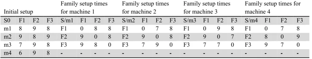
Table 3
Initial and family setup times
Family setup times for machine 4
Family setup times for machine 3 Family setup times
for machine 2 Family setup times
for machine 1 Initial setup F3 F2 F1 S/m4 F3 F2 F1 S/m3 F3 F2 F1 S/m2 F3 F2 F1 S/m1 F3 F2 F1 S0 8 7 0 F1 8 9 0 F1 8 7 0 F1 8 8 0 F1 8 9 8 m1 9 0 8 F2 7 0 9 F2 8 0 9 F2 8 0 9 F2 9 8 9 m2 0 7 9 F3 0 7 7 F3 0 9 7 F3 0 8 9 F3 8 9 7 m3 - - - - - - - - - - - - - - - - 8 9 6 m4
The number of parts for F1, F2 and F3 are 6, 5 and 2, respectively. In addition, αf for F1, F2 and F3
are 0.7, 0.19 and 0.92, respectively. Finally, due dates for F1, F2 and F3 are 160, 138 and 73, respectively. Table 4 summarizes the output results of part sequence and family sequence for the implementation of NSGAII. The six columns of Table 4 show the part sequence and the rest of the columns show the family sequence. Table 5 also summarizes the output results of part sequence and family sequence for the implementation of NRGA.
Table 4
Part sequence and part-family sequence on each family (NSGAII)
Part sequence Family sequence
F1 4 6 1 5 3 2 C1 1 3
F2 4 1 3 5 2 C2 2
F3 1 2
Table 5
Part sequence on each family (NRGA)
NRGA part sequence family sequence
F1 4 6 1 5 3 2 C1 3 1
F2 4 1 3 5 2 C2 2
F3 1 2
In order to compare the performance of NSGAII with NRGA we compare different criteria such as objective function values and CPU time. Table 6 shows the output of these results.
Table 6
The output results of NRGA and NSGAII for example
NSGAII step1 step2 NRGA Step 1 Step 2
F1 F2 F3 F1 F2 F3
Cmax 127 141 40 183.2 Cmax 127 141 40 184.2
Total Tardiness 2.5 5.6 0 120.79 Total Tardiness 2.5 5.6 0 34.794
Table 7
The output results of NRGA and NSGAII for example
NSGAII #PS = 2 S(A) = 0 C(A,B) = 0 Q(A,B) = NaN D(A)=86.0058 CPU=158.68
5.4.1 Sample problems
In this paper, sample experiments have been divided into three groups of small, medium and big problems. The number of families in small problems follow a uniform distribution at (2, 10), while their distribution is at (11, 20) and (21, 30) for medium and big problems, respectively. The number of parts in each part-family is also produced with a uniform distribution of (2, 15). The machinery for each cell is equal to 10, 20 and 30 machines for small, medium and big problems, respectively. The percentage of machine operations of each part on a machine is also produced proportion to the conditions of the problem with a uniform distribution at amplitude of (0.5, 0.9). Table 1 summarizes the results of the comparison between two algorithms in terms of different criteria.
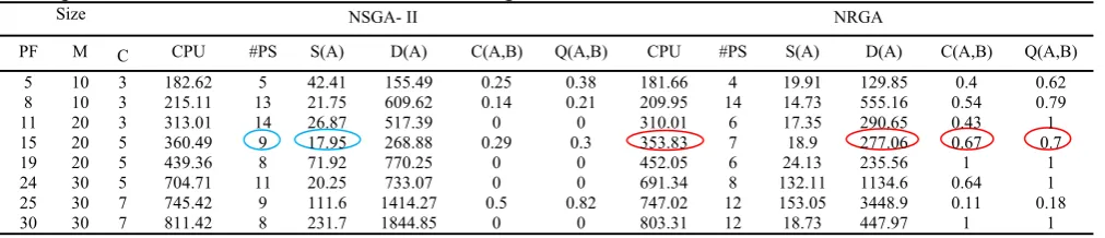
Table 8
Comparison of two methods for different examples
NRGA NSGA- II Size Q(A,B) C(A,B) D(A) S(A) #PS CPU Q(A,B) C(A,B) D(A) S(A) #PS CPU C M PF 0.62 0.4 129.85 19.91 4 181.66 0.38 0.25 155.49 42.41 5 182.62 3 10 5 0.79 0.54 555.16 14.73 14 209.95 0.21 0.14 609.62 21.75 13 215.11 3 10 8 1 0.43 290.65 17.35 6 310.01 0 0 517.39 26.87 14 313.01 3 20 11 0.7 0.67 277.06 18.9 7 353.83 0.3 0.29 268.88 17.95 9 360.49 5 20 15 1 1 235.56 24.13 6 452.05 0 0 770.25 71.92 8 439.36 5 20 19 1 0.64 1134.6 132.11 8 691.34 0 0 733.07 20.25 11 704.71 5 30 24 0.18 0.11 3448.9 153.05 12 747.02 0.82 0.5 1414.27 111.6 9 745.42 7 30 25 1 1 447.97 18.73 12 803.31 0 0 1844.85 231.7 8 811.42 7 30 30
#PS: Number of Pareto solutions, nf =(2−15)
As we can observe from Table 8, NRGA and NSGA-II produce different results. For instance, when PF=19 consists of (2-15) parts, 5 cells where each has 20 machines, based on the Pareto and distance, NSGA-II provides better solutions than NRGA but NRGA provides better than NSGA-II when we consider different criteria.
6. Conclusions
A multi-objective group scheduling problem has been provided for the cellular manufacturing system with the consideration of the learning effect. The learning effect applied for this paper is position-oriented, and Dejong learning model have been chosen for this problem. The objective functions of this problem include the minimization of the total completion time as well as the total tardiness. After offering an appropriate problem model, we have solved the resulted models by two multi-objective optimization algorithms (NSGA-II and NRGA) and their results were compared using different criteria. Future studies can focus on the objectives, limitations and parameters of the model in a phase behavior. It will also be possible to consider intercellular movements for some special parts. Investigation on cells with flexible flow shop structure in multi-objective group scheduling problem can be identified as an attractive subject for future work.
References
Al Jadaan, O., Rajamani, L., & Rao, C. R. (2008a). Non-dominated ranked genetic algorithm for
solving multi-objective optimization problems: NRGA. Journal of Theoretical and Applied
Information Technology, 4 (1), 60-67.
Al Jadaan, O., Rao, C. R., & Rajamani, L., (2008b). Improved selection operator GA. Journal of
Theoretical and Applied Information Technology, 2, 269-277.
Biskup, D., (2008). A State-of-the-art review on scheduling with learning effects. European Journal
of Operational Research, 188(2), 315-329.
Biskup, D., (1999). Single-machine scheduling with learning considerations. European Journal of
Operational Research, 115, 173-178.
Chen, P., Wu, C.-C., & Lee, W.-C., (2006). A bi-Criteria two-machine flow shop scheduling Problem
Ghosh,T., Sengupta, S., Chattopadhyay, M. & Dan, P. K. (2011). Meta-heuristics in cellular
manufacturing: A state-of-the-art review. International Journal of Industrial Engineering
Computations, 2(1), 87-122.
Deb, K., Agrawal, S., Pratap, A., & Meyarivan, T., (2000). A fast elitist non-dominated sorting
genetic algorithm for multi-objective optimization: NSGA-II. In Proceedings of the Parallel
Problem Solving from Nature VI Conference, 849–858.
Dejong, J. R., (1957). The effects of increasing skill on cycle time and its consequences for time
standards, Ergonomics, 1, 51-60.
Eren, T., & Guner, E., (2007). Minimizing total tardiness in a scheduling problem with a learning
effect. Applied Mathematical Modelling, 31, 1351-1361.
Eren, T. (2009). A bicriteria parallel machine scheduling with a learning effect of setup and removal
times. Applied Mathematical Modelling, 33, 1141–1150.
Kuo, W., & Yang, D. (2007). Single-machine scheduling with past-sequence-dependent setup times
and learning effects, Information Processing Letters, 102, 22-26.
Koulamas, C., & Kyparisis, G. J., (2007). Single-Machine and two-machine flow shop scheduling
with general learning function. European Journal of Operational Research, 178, 402-407.
Lee W.-C, & Wu C.-C, (2004). Minimizing total completion time in a two-machine flow shop with a
learning effect. International Journal of Production Economics, 88, 85-93.
Lee, W.-C, Wu, C.-C, & Sung, H.-J, (2004). A bi-criterion single-machine scheduling problem with
learning considerations. Acta Informatics, 40, 303-315.
Lee, W-C., & Wu, C.-C. (2009). A note on single-machine group scheduling problems with
position-based learning effect. Applied Mathematical Modelling. 33(4), 2159-2163.
Logendran, R., Salmasi, N., & Sriskandarajah, C., (2006).Two-machine group scheduling problems
in discrete parts manufacturing with sequence-dependent setups. Computers & Operations
Research, 33, 158-180.
Mosheiov, G., (2001a). Scheduling problems with a learning effect. European Journal of Operational
Research, 132, 687-693.
Mosheiov, G., (2001b). Parallel machine scheduling with a learning effect. Journal of the
Operational Research Society, 52, 1-5.
Nanda, R., & Alder, G. L., (1982). Learning curves: theory and application, Atlanta: Industrial
Engineering & Management Press.
Schaller, J.E., Gupta, J.N.D., & Vakharia, A.J., (2000). Scheduling a flow line manufacturing cell
with sequence dependent family setup times. European Journal of Operational Research, 125(2),
324-339.
Wang, J., & Xia, Z., (2005). Flow-shop scheduling with a learning effect. Journal of the Operational
Research Society, 56(4), 1325-1330.
Wu, C-C., & Lee, W-C., (2009). Single-machine and flow shop scheduling with a general learning
effect model. Computers & Industrial Engineering, 56(4), 1553-1558.
Zegordi, S.H., Itoh, K., & Enkawa, T., (1995). A knowledge simulated annealing scheme for the
early/tardy flow shop scheduling problem. International Journal of Production Research, 33(5),
1449-1466.
Zitzler, E., & Thiele, L., (1999). Multi objective evolutionary algorithms: a comparative case study
and the strength Pareto approach. IEEE Transactions on Evolutionary Computation, 4(3),
257-271.
Zitzler, E., Deb, K., & Thiele, L., (2000). Comparison of multi objective evolutionary algorithms. Evolutionary Computation journal. 8(2), 125-148.
Zhao, C.-L., Zhang, Q.-L., & Tang, H.-Y. (2004). Machine scheduling problems with learning
effects. Dynamics of Continuous, discrete and Impulsive Systems, Series A: Mathematical