A Basic Period Approach for Solving the Economic Lot and Delivery Scheduling in Flexible Flow Lines

A BASIC PERIOD APPROACH FOR SOLVING

THE ECONOMIC LOT AND DELIVERY SCHEDULING

IN FLEXIBLE FLOW LINES

S.A. Torabi*

Department of Industrial Engineering, College of Engineering, University of Tehran P.O. Box 11155/4563, Tehran, Iran

[email protected]

M. Jenabi

Department of Industrial Engineering, Amirkabir University of Technology P.O. Box 15916-343, Tehran, Iran

[email protected]

*Corresponding Author

(Received: October 9, 2007 – Accepted in Revised Form: May 9, 2008)

Abstract In this paper, the problem of lot sizing, scheduling and delivery of several items in a two-stage supply chain over a finite planning horizon is studied. Single supplier via a flexible flow line production system (FFL), produces several items and delivers them directly to an assembly facility. Based on basic period (BP) strategy, a new mixed zero-one nonlinear programming model has been developed with the objective of minimizing the average setup, inventory-holding and delivery costs per unit time in the supply chain without any stock-out. The problem is very complex and it can not be optimaly solved, especially in real-sized problems. So, an efficient hybrid genetic algorithm (HGA) has been proposed based on applying, the most applied BP approach i.e. power-of-two policy. Based on some problem instances, the solution quality of the algorithm has been evaluated and also compared with the common cycle approach. Numerical experiments demonstrate the effectiveness of the proposed HGA.

Keywords Flexible Flow Lines, Lot and Delivery-Scheduling, Basic Period Approach, Power-of-Two Policy, Hybrid Genetic Algorithm (HGA)

ﻩﺪﻴﻜﭼ

ﺍﺭﺩ ﻳ ﻌﺗﻪﻠﺌﺴﻣﻪﻟﺎﻘﻣﻦ ﻴﻴ

ﻟﻮﺗﯼﺪﻨﺑﻥﺎﻣﺯﻭﯼﺩﺎﺼﺘﻗﺍﯼﺎﻫﻪﺘﺷﺎﺒﻧﺍﻩﺯﺍﺪﻧﺍﻦ ﻴ

ﻮﺤﺗﻭﺪ ﻳ ﺭﺩﺎﻬﻧﺁﻞ ﻳ

ﺠﻧﺯﮏ ﻴ ﻩﺮ

ﻣﺎﺗ ﻴ ﯽﻃﯽﺤﻄﺳﻭﺩﻦ ﻳ

ﯽﻣﯽﺳﺭﺮﺑﺩﻭﺪﺤﻣﻖﻓﺍﮏ ﺩﻮﺷ

. ﺍﺭﺩ ﻳ ﺠﻧﺯ ﻦ ﻴ ﻩﺮ ﻳ ﻣﺎﺗﮏ ﻴ ﻦ ﺭﺩﺍﺭﯽﻔﻠﺘﺨﻣﺕﻻﻮﺼﺤﻣﻩﺪﻨﻨﮐ

ﻳ ﺳﮏ ﻴ ﻟﻮﺗﻢﺘﺴ ﻴ ﺮﺟﺪ ﻳ ﻟﻮﺗﻂﻠﺘﺨﻣﯽﻫﺎﮔﺭﺎﮐﻥﺎ ﻴ

ﻘﺘﺴﻣﺭﻮﻄﺑﻭﺪ ﻴ

ﻮﺤﺗﻢ ﻳ ﻞ ﻳ ﯽﻣﺮﮔﮊﺎﺘﻧﻮﻣﮏ ﺪﻫﺩ

. ﯼﺯﺎﺳﻝﺪﻣﯼﺍﺮﺑ

ﺍﻳ ﺳ ﺯﺍ ﻪﻠﺌﺴﻣ ﻦ ﻴ

ﻥﺎﻣﺯ ﺖﺳﺎ ﺳ ﯼﺪﻨﺑ

ﻴ ﺎﭘ ﻞﮑ ﻳﻪ ﻭ ﻩﺩﺎﻔﺘﺳﺍ ﻳ

ﻏ ﻝﺪﻣ ﮏ ﻴﺮ

ﺤﺻ ﺩﺪﻋ ﻂﻠﺘﺨﻣ ﯽﻄﺧ ﻴ

ﻑﺪﻫ ﺎﺑ ﺢ

ﻞﻗﺍﺪﺣ ﺰﻫ ﻉﻮﻤﺠﻣﯼﺯﺎﺳ ﻳ

ﻩﺍﺭﯼﺎﻫ ﻪﻨ ﻮﺤﺗ ﻭﯼﺭﺍﺪﻬﮕﻧ،ﯼﺯﺍﺪﻧﺍ

ﻳ ﺠﻧﺯ ﻞﮐﺭﺩﻞ ﻴ

ﯽﻣﻪﺋﺍﺭﺍﻩﺮ ﺩﻮﺷ

. ﻟﺪﺑ ﻴ ﻥﺎﮑﻣﺍ ﻡﺪﻋﻞ

ﻘﺘﺴﻣﻞﺣ ﻴ ﺍﻢ ﻳ ﺭﻝﺪﻣﻦ ﻳ ﯽﻌﻗﺍﻭﺩﺎﻌﺑﺍﺎﺑﻞﺋﺎﺴﻣﯼﺍﺮﺑﯽﺿﺎ ،

ﻳ ﺭﻮﮕﻟﺍﮏ ﻳ ﺘﻧﮊﻢﺘ ﻴ ﮐﺮﺗﮏ ﻴ ﺳﻦﺘﻓﺮﮔﺮﻈﻧﺭﺩﺎﺑﯽﺒ ﻴ

ﺖﺳﺎ

ﻥﺍﻮﺗ ﺩﺪﻋﯼﺎﻫ ﻪﻌﺳﻮﺗﻭﺩ ﻳ

ﺎﺘﻧﻭﻪﺘﻓﺎ ﻳ ﺑﯼﺩﺪﻋﺕﺎﺒﺳﺎﺤﻣﺞ ﻴ

ﺍﺭﺎﮐﺮﮕﻧﺎ ﻳ ﺍﯽ ﻳ ﺎﻘﻣﺭﺩﺵﻭﺭﻦ ﻳ

ﺳﺎﺑﻪﺴ ﻴ ﻥﺎﻣﺯﺖﺳﺎ ﯼﺪﻨﺑ

ﺳ ﻴ ﺖﺳﺍﮎﺮﺘﺸﻣﻞﮑ .

1. INTRODUCTION

Nowadays, there is a great tendency to develop integrated models in research community for simultaneously cost-effective planning of different activities in supply chains. Among them, integrated production and delivery planning between adjacent supply parties is of particular interest which can

continuously. Researches on the ELSP usually focus on cyclic schedules (i.e., schedules that are repeated periodically) with three well known policies: common cycle, basic period (or multiple cycle) and time varying lot size approaches (Torabi, et al [1]). Several authors have extended the ELSP to multistage production systems with common cycle production policy [e.g., 2-9].

The economic lot and delivery-scheduling problem (ELDSP) is an extension of ELSP to a two-stage supply chain where a supplier produces several items for an assembly facility and delivers them in a static condition. Hahm, et al [10,11] provided an excellent review of models related to ELDSP and developed two efficient heuristic algorithms to solve, based on common cycle and nested schedule strategies, respectively. Jensen, et al [12] developed an optimal polynomial time algorithm for the ELDSP under common cycle approach. Finally, Torabi, et al [5] considered the ELDSP in flexible flow lines under common cycle approach and over a finite planning horizon. They developed an effective HGA to obtain near (or ideally optimal) solutions.

Regarding the basic period (BP) approach, Bomberger, et al [13] assumed different production cycles for items in which each cycle time must be an integer multiple of a BP that is long enough to meet the demand of all items. The production frequency of each product during the global cycle is then determined as a multiple of the selected BP. In such a case, infeasibility results from the artificial restrictions are imposed by the concept of BP. Elmaghraby, et al [14] provided a review of the various contributions to ELSP and presented an improvement upon the BP approach, called extended basic period (EBP) method. Its main difference from Bomberger’s BP method was that it allowed items to be loaded on two BPs simultaneously and at the same time relaxed the requirement that, the basic period should be large enough to accommodate such simultaneous loading. Yao, et al [15] developed an evolutionary algorithm for ELSP under basic period policy. Also, Ouenniche, et al [16-18] proposed three efficient heuristic approaches, i.e. power of two, two groups and G-group methods for the ELSP in a flow shop systems over an infinite planning horizon under basic period approach.

In all the above works, the planning horizon is

assumed to be infinite. However, this assumption considerably reduces the usefulness of the proposed contributions, because in practice, planning horizon is often finite. In this regard, there are few research works which have assumed the finite planning horizon [1,2,5,19].

Consequently, to the best of our knowledge, there is no research on ELDSP in flexible flow lines under basic period approach over a finite planning horizon so far. It is noted that the solutions obtained via the basic period approach are generally better than the common cycle's solutions, and this is our main motivation in this research work.

In this paper we have studied the finite horizon economic lot and delivery scheduling problem in flexible flow lines under basic period approach. At first, a new mixed zero-one nonlinear program has been developed whose optimal solution simultaneously determines; the optimal assignment of products in basic periods, optimal assignment of products to machines at stages with multiple parallel machines, the optimal products sequence for each machine at each stage, the optimal lot sizes and the optimal production and delivery schedule at each global cycle.

To solve the problem, we assume that the cycle time of product i, Ti, is an integer multiple, say ki,

of a basic period F; i.e. Ti = ki.F for all i. In

addition we are required that the basic period F to be such that the planning horizon PH is an integer multiple of a global cycle H.F; that is PH = r.H.F where r is an integer and H denotes the least common multiple (LCM) of the ki’s.

Consequently, to solve the problem, a hybrid genetic algorithm (named PT-HGA) has been proposed based on power of two policy (the most applied BP strategy).

The outline of the paper is as follows: problem formulation has been presented in Section 2. The proposed HGA have been explained in Section 3. In Section 4, an efficient procedure has been developed for determining upper bounds on ki

2. PROBLEM FORMULATION

The following assumptions are considered for the problem formulation:

• Machines at stages with multiple parallel machines are identical (in all characteristics such as production rates and setup times/cost) • Machines of different stages are continuously available and each machine can only process one product at a time.

• At stages with parallel machines, each product is processed entirely on one machine.

• Setup times/costs in supplier's production system are sequence independent.

• Production sequence at each basic period for each machine at each stage is unique and is determined by the solution method.

• The supplier incurs linear inventory holding costs on semi-finished products.

• Both the supplier and the assembler incur linear holding costs on end products.

• Preemption/Lot-splitting is not allowed. Moreover, the notations used for the problem formulation are defined as follows:

Parameters

n Number of products

m Number of work centers (stages) mj Number of parallel machines at stage j

Mk'j K'-th machine at stage j

di Demand rate of product i

pij Production rate of product i at stage j

sij Setup time of product i at stage j

scij Setup cost of product i at stage j

hij Inventory holding cost per unit of product i

per unit time between stages j and j+1

hi Inventory holding cost per unit of final

product i per unit time

A transportation cost per delivery PH Planning horizon length M A large real number

Decision Variables

σk Sequence vector in basic period k

σkk'j Sequence vector of machine Mk'j related to

the basic period k

r Number of production cycles over the finite planning horizon

nkk'j Number of products assigned to machine

Mk'j related to the basic period k

F Basic period length

bij Production beginning time of product i at

stage j (after related setup operation) ki Time multiple of product i

⎪ ⎪ ⎪ ⎩ ⎪⎪ ⎪ ⎨ ⎧

′ −

= ′

. Otherwise ,

0

j k M of position th

the to

assigned is

k period basic at i product If , 1

kj k i

x _l

l

It is noted that based on above variables, the global cycle length is equal to the least common multiple of the ki variables, in other words we would have:

H = LCM (k1, k2,…,kn). Also, the production cycle

length, the production lot size of product i and the processing time for a lot of product i at stage j would be as follows:

Ti = ki.F, Qi = di.Ti, ptij= Qi /pij =di.ki.F / pij.

Moreover, at stages with only one machine the value of mj and index k' would be only one. Since

after processing each product at each stage, there would be a value added for the product, values of hij

parameters will be non-decreasing; that is hi,j-1≤ hij.

The objective function of this problem (Problem P) includes two fundamental expressions. First expression is related to the setup and transportation costs. This expression consists of two parts: the first part computes the setup cost of products with respect to their production cycle times. The second part computes the transportation cost of products on each basic period.

. n

1 i

m 1

j F

A F i k

ij sc

C ∑

= ∑= +

=

The inventory holding costs are often more complicated which are incurred at both the supplier and the assembler. Figure 1 shows the inventory level of final product i in one cycle at the assembly facility is d_iT_i 2

2i T i T i d i T

1 ₌

⎟ ⎟ ⎠ ⎞ ⎜

⎜ ⎝ ⎛

time

Ti

i

I

i i .T

d

Figure 1. Inventory level at the assembler in one cycle.

time

ij i i ij d.k.F p

b +

1 j ,i i i 1 j ,

i d.k.Fp

b ₋ + ₋

1 j , i

b ₋ b_ij

i i .T

d 1 j ,i

WIP ₋

Figure 2. WIP between stages j-1 and j at the supplier.

im i i

im d .k F p

b +

time

i

I

i i .T

d

im

b Ti

Figure 3. Final product inventory at the supplier.

the assembly facility will be:

∑ = n 1 i hikidi 2

F

Two types of inventories i.e. WIP and finished product inventories are considered for the supplier. Figures 2 and 3 show the evolution of WIP inventory of product i between two successive stages j-1 and j, and the inventory level of final product i, respectively.

From Figure 2 it is obvious that the average WIP inventory of product i between two successive stages j-1 and j per unit time is:

. 1 j ,i p 2

F i k i d 1 j ,i b ij p 2

F i k i d ij b i d

ij p

i T i d 2

i T i d 1 j ,i p

i T i d 1 j ,i b ij b i T i d 1 j ,i p

i T i d 2

i T i d i T 1

1 j ,i I

⎟⎟ ⎟

⎠ ⎞

⎜⎜ ⎜

⎝ ⎛

− − − − + =

⎪⎭ ⎪ ⎬ ⎫ +

⎟⎟ ⎟

⎠ ⎞

⎜⎜ ⎜

⎝ ⎛

− − − − ⎪⎩

⎪ ⎨ ⎧

Therefore, the total WIP inventory holding cost for all products per unit time at the supplier would be as follows: . 1 j ,i p 2 F i k i d 1 j ,i b ij p 2 F i k i d ij b i d n 1 i m 2 j ,ij 1

h WIP TC ⎪⎭ ⎪ ⎬ ⎫ − − − ⎪⎩ ⎪ ⎨ ⎧ − + ∑ = ∑= − =

Also, from Figure 3, we can derive the average inventory of final product i per unit time:

. im b i d F i k im p 2 i d . 1 i d im p i T i d im b i T i T i d im p i T i d . 2 T i d T 1 1 j , i I − ⎟ ⎟ ⎠ ⎞ ⎜ ⎜ ⎝ ⎛ − = ⎪⎭ ⎪ ⎬ ⎫ ⎟ ⎟ ⎠ ⎞ ⎜ ⎜ ⎝ ⎛ − − ⎪⎩ ⎪ ⎨ ⎧ + = −

Thus, the total inventory holding cost for all final products per unit time is:

. im b . i d n 1 i . i h F i k . ikm p . 2 i d 1 i d n 1 i . i h FI TC ∑ = − ⎟ ⎟ ⎠ ⎞ ⎜ ⎜ ⎝ ⎛ − ∑ = =

So, the total cost per unit time (i.e. objective function of Problem P) would be as follows:

. n

1 i hidibim n

1 i

m 2

j h,ij 1.di bij b,ij 1 m

2

j p,ij 1

1 ij p 1 1 j ,i h . 2 2 i d n 1

i pim

i d 3 . 2 i k . i d . i h . F n 1 i m 1 j kiF

ij sc F A TC ∑ = − ∑ = ∑= ⎟⎠ ⎞ ⎜ ⎝ ⎛ − − − + ⎥ ⎥ ⎥ ⎦ ⎤ ∑ = ⎟⎟ ⎟ ⎠ ⎞ ⎜⎜ ⎜ ⎝ ⎛ − − − ∑ = ⎢ ⎢ ⎣ ⎡ + ⎟ ⎟ ⎠ ⎞ ⎜ ⎜ ⎝ ⎛ − + ∑ = ∑= + =

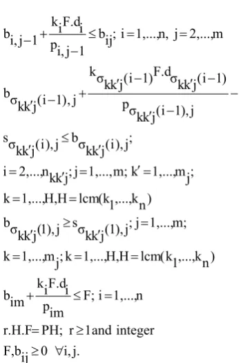
Regarding this objective function and logical relationships between variables of Problem P (that some of them are recognizable from inventory level curves), a mixed zero-one nonlinear model is developed to obtain optimal solution of the problem.

Problem P has the following set of constraints. Constraints (2) state that no product can be processed before it is completed at previous stage.

Constraints (3) show that, no product can be processed before the completion of its predecessor in the related production sequence (σkk'j). Constraints (4) reveal that at each position

of each machine, there is at most one product; because for each machine such as Mk'j, may

assigne less than n products. Constraints (5) state that one product can be assigned at one position of machine Mk'j; if another product is to be

assigned at the previous position of this machine. Constraints (6) ensure assignment of product i to one of the first ki basic period and implies that

each assigned product at each stage has a unique position in the sequence of one machine. Constraints (7) determine assignment of products in appropriate basic periods during the H basic periods. Constraints (8) denote that if product i has been assigned to basic period k at stage j, it must be assigned to that basic period at all stages. Constraints (9) show that if product i is the first product in the sequence vector of one machine at stage j, it’s processing cannot be started before setting up the corresponding machine. Constraints (10) assure that the resulting schedule is cyclic so that the process completion time for each product at final stage is less than or equal to a basic cycle time F. Constraint (11) implies that the planning horizon PH is an integer multiple of H.F, where H = LCM (k1,…,kn), and F is the basic period

length. Constraints (12) show that r is an integer greater than or equal to one. Finally, Constraints (13) are the non-negativity constraints of variables.

. n

1 i hidibim n

1 i

m 2

j h,ij 1di bij b,ij 1 m

2

j p,ij 1

1 ij p 1 1 j ,i h 2 2 i d i k n 1

i pim

i d 3 2i k . i d i h F n 1 i m 1 j kiF

ij sc F A Z Min : P Problem ∑ = − ∑ = ∑= ⎟⎠ ⎞ ⎜ ⎝ ⎛ − − − + ⎥ ⎥ ⎥ ⎦ ⎤ ∑ = ⎟⎟ ⎟ ⎠ ⎞ ⎜⎜ ⎜ ⎝ ⎛ − − − + ∑ = ⎢ ⎢ ⎣ ⎡ ⎟ ⎟ ⎠ ⎞ ⎜ ⎜ ⎝ ⎛ − + ∑ = ∑= + = Subject to m ,..., 2 j ; n ,..., 1 i ; ij b 1 j ,i p F i k i d 1

i,j-b ≤ = =

−

(

)

n k ,..., 1 k cm l H , H ,..., 1 k ; n ; j m ,..., 1 k ; m ,..., 1 j ; i u , n ,..., 1 i ; kj k 1 u x kj k i x 2 M uj b ij s ij p F i k i d ij b ⎟ ⎠ ⎞ ⎜ ⎝ ⎛ = = < = ′ = ≠ = ⎟ ⎠ ⎞ ⎜ ⎝ ⎛ ′ + − ′ − ≤ − + + l l l (3) ⎟ ⎠ ⎞ ⎜ ⎝ ⎛ = = = = ′ = ≤ ∑ = ′ n k ,..., 1 k lcm H , H ,..., 1 k ; n ,..., 1 ; j m ,..., 1 k ; m ,..., 1 j ; 1 n 1 i i kkj

x l l (4)

( )

⎟ ⎠ ⎞ ⎜ ⎝ ⎛ = = < = = = ∑ = ′ ≤ ∑ = + ′ n k ,..., 1 k cm l H , H ,..., 1 k ; n ; j m ,..., 1 k ; m ,..., 1 j ; n ,..., 1 i ; n 1 u u kkj

x n

1

i i 1kkj x l l l (5) m ,..., 1 j ; n ,..., 1 i ; 1 j m 1 k n 1 i k 1 k i kkj

x = = =

∑ =

′ _l∑= ∑= l ′ (6)

(

)

2 i k H ,..., 0 b ; i k ,..., 1 t ; m ,..., 1 j ; n ,..., 1 i ; j m 1 k n

1 i k t b 1ki j x j m 1 k n

1 i k t bki j x − = = = = ∑ = ′ ∑= ′ + + = ∑ = ′ ∑= ′ + ⎟ ⎠ ⎞ ⎜ ⎝ ⎛ ⎟ ⎠ ⎞ ⎜ ⎝ ⎛ l l l l (7) H ,..., 1 k ; m j , m ,..., 1 j ; m ,..., 1 i ; j m 1 k n

1xilkk,j 1 j

m

1 k

n

1xilkkj

= < = = ∑ = ′ ∑= ′ + = ∑ =

′ _l∑= ′ _l (8)

⎟ ⎠ ⎞ ⎜ ⎝ ⎛ = = = = ⎟ ⎟ ⎟ ⎠ ⎞ ⎜ ⎜ ⎜ ⎝ ⎛ ∑ = ′ ′ − − ≥ n k ,..., 1 k cm l H , H ,..., 1 k ; n ,..., 1 i , m ,..., 1 j ; j m 1 k i1kkj

x 1 M ij s ij b (9) , n ,..., 1 i ; F im p F i k i d im

b + ≤ = (10)

⎟ ⎠ ⎞ ⎜ ⎝ ⎛ =

=PH;H lcm k₁,...,k_n

H.F.r (11)

r and Intege

, 1

r≥ (12)

{ }

0,1; ,i ,k, ,jk.

kj k i x ;j ,i 0 ij b ; 0

F≥ ≥ ∀ _{l ′} = ∀ _l ′ (13)

It is noted that this model can be run for a set of known ki variables. In other words, to run this

model, at first the ki values must be determined,

and then the corresponding optimal basic period length, optimal assignments, sequence vectors and production and delivery schedule of products are obtained via solving Problem P.

3. Proposed hybrid genetic algorithm

During the last thirty years, there has been a growing interest in obtaining the optimal solutions for complex systems using genetic algorithms (GA). Genetic algorithms maintain a population of potential solutions and simulate evolution process using some selection process based on fitness of chromosomes and some genetic operators. To improve solution quality and to escape from converging to local optima, various strategies of hybridization have been suggested [5,20]. In designing a hybrid genetic algorithm (HGA), the neighborhood search (NS) heuristic usually acts as a local improver into a basic GA loop.

In our HGA, each solution is characterized with a set of ki multipliers and the value of basic period

F. Beside the cost minimization; we have to generate feasible schedules. Therefore, a capacity feasibility test has been developed in Section 5 which is able to identify the infeasible solutions and converting them to feasible schedules.

3.1. Chromosome Representation

The proposed HGA search in the solution space of ki

values, so that each chromosome is a binary (zero-one) string, and each ki multiplier will be

represented as a particular part of a chromosome. For instance, the first u1 bits are used to encode the

value of k1 and the particular piece of chromosome

from the (u1+1)-th bit to the (u1+u2)-th bit

represents the value of k2 and so on. In order to

represent all the possible values of ki for each item

encoding the value of ki into a binary string, we

have to establish a mapping between each binary string and an integer ki. In fact, we map a binary

string consisting of ui bits to an integer value ki by

using the following equations for the power of two and non-power of two cases, respectively:

i v 2 i k 10 i v 10 i

u

1 j

1 j 2 j b

2 1 b ... 1 i u b i u b

= ⇒ ⎟ ⎠ ⎞ ⎜ ⎝ ⎛ = ⎟⎟ ⎟

⎠ ⎞

⎜⎜ ⎜

⎝ ⎛

∑ =

−

= −

3.2. Determining The

σ

k

Vectors

In assigning and sequencing of products in different basic periods i.e. determination of σk vectors, it is not

easy to derive a simple necessary and sufficient condition to have a non-empty set of feasible solutions. Given a vector of multipliers ki; i =

1,…,n, the procedure starts to make a vector say V' by sorting the products in ascending order of ki

and, within the products having the same multiplier ki , in the descending order of ρi where:

∑

= =

=

ρ m

1 j

. n ..., , 1 i , ij p

i d i k i

Each product i in the vector V' is assigned to the basic period t within the first ki periods of global

cycle H which minimizes:

⎪ ⎭ ⎪ ⎬ ⎫

⎪ ⎩ ⎪ ⎨ ⎧

⎟ ⎟ ⎟

⎠ ⎞

⎜ ⎜ ⎜

⎝ ⎛

+ ∑

σ ∈ =

+

= p_iji

d i k

k u puj

u d u k m

,..., 1 j

maximum ,...

i m t,t kmaximum

Finally, for each k, k=1,…,H, we determine the sequence of products within σk such that if i, u ∈ σk and i is ordered before u in V', then i also is

ordered before u in σk.

3.3. Determining the

σ

kk'j

Vectors

First available machine (FAM) rule has been employed to assign and sequence the products of each basic period to machines of different stages (Torabi, et al [5]. According to this procedure, for any given permutation vector V; the products are assigned to machines of first stage by using FAM rule (if m1 >

1). Then, for each of subsequent stages, the products

have been first sequenced according to increasing order of their process completion time at the previous stage, and then assigned to the machines at the current stage according to FAM rule.

3.4. Initial Population

Initial population of binary chromosomes is generated randomly. According to feasibility test, each infeasible solution is converted to a feasible one and then is inserted into the initial population.

3.5. Evaluation Function

Each chromosome in the population represents a potential solution to the problem. Evaluation function is responsible for rating these potential solutions by assigning a real number as a measure of their fitness. In our problem after determining the σkk'j vectors for each

chromosome, evaluation function is obtained by solving the following NLP model (Problem P1). This problem is derived from Problem P by substituting xilkk'j values by corresponding ones.

Also, σkk'j(i) indicates the i-th product in the

sequence vector of machine Mk'j in basic period k.

Problem P1 can be solved by the following iterative procedure:

Initial step. Let r = 1, and solve the resultant linear program.

Iterative step. Increase r by 1 and solve the corresponding linear program for this new value of r. If this model has no feasible solution, stop; else, if the objective function for current value of r (i.e. Zr) is less than this

value for previous r (i.e. Z), then set Z = Zr and F* = PH/r.H, and go

to the next iteration.

Problem P1:

∑ = − ∑

= ∑= ⎟⎠

⎞ ⎜

⎝ ⎛

− − −

+ ⎥ ⎥ ⎥ ⎦ ⎤

⎟⎟ ⎟

⎠ ⎞

⎜⎜ ⎜

⎝ ⎛

− − ∑

= −

∑ = ⎢

⎢ ⎣ ⎡

+ ⎟ ⎟ ⎠ ⎞ ⎜

⎜ ⎝ ⎛

− +

∑ = ∑= + =

n

1

i im

.b i .d i h n

1 i

m

2

j i,j 1

b ij b i .d 1 j i, h

F 1 j i, p

1 ij p

1 m

2

j 2

2 i d . i .k 1 j i, h

n

1

i pim

i d 3 2i d . i .k i h n

1 i

m

1 j kiF

ij sc F

Figure 4. Two-point crossover.

Subject to:

j. i, 0 ij b F,

integer and 1 r PH; r.H.F

n 1,..., i F; im p i

F.d i k im b

) n k ,..., 1 k ( lcm H H, 1,..., k ; j m 1,..., k

m; 1,..., j ; j ), 1 ( j k k σ s j ), 1 ( j k k σ b

) n k ,..., 1 (k lcm H H, 1,..., k

; j m 1,..., k m; 1,..., j ; j k k n 2,..., i

; j ), i ( j k k σ b j ), i ( j k k σ s

j ), 1 i ( j k k σ p

) 1 i ( j k k σ F.d ) 1 i ( j k k σ k

j , ) 1 i ( j k k σ b

m 2,..., j n, 1,..., i ; ij b 1 j i, p

i F.d i k 1 j i, b

∀ ≥

≥ =

= ≤ +

= =

=

= ′

≥ ′

= =

= ′ =

′ =

′ ≤ ′

− −

′

− ′ −

′ + − ′

= =

≤ − + −

3.6. Selection and Crossover Operators

In proposed HGAs, we have used the tournament selection approach. It randomly chooses two chromosomes from parent pool, and then chooses the fittest one if a random value generated (τ) is smaller than a pre-set probability value φ (0.5<φ< 1). Otherwise, the other one is chosen. Then, the selected chromosomes are duplicated and pairs of them are selected as parents to undergo the crossover operation.

The main purpose of crossover is to exchange genetic materials between randomly selected parents with the aim of producing better offspring. In this research we have used the classic two point crossover based on the results obtained from the initial tests. According to this crossover, at first two positions are randomly selected, and then the

genes between them in the parent chromosomes are exchanged (see Figure 4).

3.7. Mutation Operator

Mutation introduces random variation (diversification) into the population. Most genetic algorithms incorporate mutation operator mainly to avoid convergence to local optima in the population and recovering lost genetic materials. In the proposed HGAs, we have used the swap mutation. Figure 5 illustrates an example of this operator.

3.8. Local Improver

Our local improvement procedure is based on an iterative neighborhood search (NS) so that within successive interchanges, given offspring is replaced with an elite (dominating) neighbor. We have used inversion operator as local improver. Figure 6 is an example of this operator.

3.9. Population Replacement

Chromosomes for the next generation are selected from the enlarged population. After offspring were generated from GA operators (crossover and mutation) and then improved by the neighborhood search procedure, the improved offspring are added to the current population. This population is called the enlarged population, and then about 60 percent of the new population is filled out by the best and the fittest chromosomes of the enlarged population. Remaining chromosomes are selected randomly from the remainder chromosomes in the enlarged population.

Figure 5. Swap mutation.

Figure 6. Inversion operator.

executed or the pre-set number of generations without any improvement in the last best solution, max_nonimprove, reaches.

4. DETERMINING UPPER BOUNDS ON ki

VALUES

In order to represent all possible and feasible values of each ki multiplier, we determine an upper

bound for each one. In our HGAs, we derive an upper bound on ki through determining an upper

bound on the objective value of each product i. Following steps describe how we can compute an upper bound for each ki (kiUB):

Step 1.

For each product i, assume ki= 1 and

calculate ∑j di/pij, arrange the products in ascending

order of these values. Assign the products and sequence them to machines at all stages via FAM rule. Finally, find the corresponding common cycle solution and its objective function, TCcc.

Step 2.

Calculate the cost share of each product i,

∑ _{= ≠}

−

=TC_cc n_{u 1,u i}TCu_cc i

cc

TC . As it had been

mentioned by Yao, et al [15], we would have: TCi

BP≤ TCicc, where TCiBP is cost share of product

i under basic period approach. So, TCi

BP values

must be determined.

Step 3.

Assume there is only one product (say

product i) with following objective function:

. im b i d i h m 2

j h,ij 1.di bij b,ij 1 m

2

j p,ij 1

1 ij p 1 1 j ,i h . 2 2 i d i k im p i d 3 . 2 i k . i d . i h . F m 1 j kiF

ij sc i BP TC − ∑ = ⎟⎠ ⎞ ⎜ ⎝ ⎛ − − − + ⎥ ⎥ ⎥ ⎦ ⎤ ∑ = ⎟⎟ ⎟ ⎠ ⎞ ⎜⎜ ⎜ ⎝ ⎛ − − − + ⎢ ⎢ ⎣ ⎡ ⎟ ⎟ ⎠ ⎞ ⎜ ⎜ ⎝ ⎛ − + ∑ = =

Obviously, to obtain the optimal solution, we have to determine the starting times so that minimize

(bij-bi,j-1)-bim. Also, the smallest feasible value of

bij-bi,j-1 is equal to kiF.di/pi,j-1. Therefore, the best

value of TCi

BP is equal to:

∑− = − ⎥ ⎥ ⎥ ⎦ ⎤ ⎢ ⎢ ⎢ ⎣ ⎡ ∑ = ⎟⎟ ⎟ ⎠ ⎞ ⎜⎜ ⎜ ⎝ ⎛ − + − + ⎟ ⎟ ⎠ ⎞ ⎜ ⎜ ⎝ ⎛ − + ∑ = = 1 m 1 j pij

1 2 i d i h m 2

j p,ij 1

1 ij p 1 1 j ,i h . 2 2 i d im p i d 3 . 2i d . i h . F i k m 1 j kiF

ij sc i

BP TC

Finally for a given value of F, we can derive an upper bound on vi, (k_i =2vi), denoted by viUB by

using following equations:

. min F . i H 2 m 1 j ij sc i H 4 2 i cc TC i cc TC 2 log UB i v 0 m 1 j scij i cc TC . F i k i H 2 F 2 i k i cc TC i H . F i k m 1 j kiF

ij sc i cc TC i BP TC ⎥ ⎥ ⎥ ⎥ ⎥ ⎥ ⎥ ⎦ ⎤ ⎢ ⎢ ⎢ ⎢ ⎢ ⎢ ⎢ ⎣ ⎡ ⎟ ⎟ ⎠ ⎞ ⎜ ⎜ ⎝ ⎛ ∑ = − ⎟ ⎠ ⎞ ⎜ ⎝ ⎛ + = ⇒ ≤ ∑ = + − ⇒ ≤ + ∑ = ⇒ ≤ Where ∑ = ⎟⎟ ⎟ ⎠ ⎞ ⎜⎜ ⎜ ⎝ ⎛ − + − + ⎟ ⎟ ⎠ ⎞ ⎜ ⎜ ⎝ ⎛ − = m 2

Moreover, to determine the minimum value of F, Fmin, assume that F must be large enough so that at

least one product with ki = 1, can be produced

during it. Consequently, Fmin is obtained from the

following equation:

. m

1 j di pij 1

m 1 j sij n

,..., 1 i

maximum F

F m

1 j pij

F i d m

1 j sij n

,..., 1 i

maximum

⎪⎭ ⎪ ⎬ ⎫

⎪⎩ ⎪ ⎨ ⎧

∑ = −

∑ = =

≥ ⇒

≤ ⎪⎭ ⎪ ⎬ ⎫

⎪⎩ ⎪ ⎨ ⎧

∑ = + ∑ = =

5. FEASIBILITY TEST AND REPAIR PROCEDURE

For a given chromosome and related ki, σk and σkk'j

vectors, a simple test for capacity feasibility can be carried out. To do so, the process completion times of products for all H basic periods are first calculated. We can use the following procedure for doing so.

Then, if at least at one basic period, the related completion time would be greater than or equal to 1, the corresponding chromosome is infeasible and otherwise, it is feasible. In other words, if at least one of the ftk values, k = 1,…, H, be greater than or

equal to 1, this solution would be infeasible. for k = 1,…,H

for each i ∈σk

for j = 1,…,m

. 1 j , k M machine on k period

basic at i before is u product

; 1 j ,i p

i d i k

1 j , k k

u pu,j 1 u d u k 2

process

, j k M machine on k period

basic at i before is u product

; j

k k

u k_ud_u p_uj 1

process

− ′

− + ∑

− ′ σ

∈ −

=

′ ∑

′ σ ∈ =

fin = max{process1,process2} + kidi /pij

end ftik = fin

end

ftk = maxi{ftik}

end

For converting an infeasible solution to a feasible one, we have also proposed following iterative repair procedure based on ki values modifications.

Step 1.

Choose the basic period with maximal value of ftk, e.g. basic period k1.

Step 2.

Among the products of basic period k1, select the product with maximum amount of process time (maxi {∑j = 1,…,m kidi/ pij}; i ∈σk1), e.g.

product i.

Step 3.

If vi ≠ 0; set vi = vi -1, and obtain σk and σkk'j vectors for this new set of multiples. If this

solution is feasible, stop, otherwise go to step1. If vi = o; select the product with subsequent

maximum amount of process time and go to step 3. It is noteworthy that each chromosome obtained via genetic operators (crossover, mutation and local improver) is checked with aforementioned feasibility test.

6. COMPUTATIONAL EXPERIMENTS

However, because of the confidentiality as well as the lack of some required data, we decided to generate random problem instances.

6.1. Parameter Setting and Data Set

The tuned parameters of the HGA after some initial tests have been adjusted as: population size pop_size = n, maximum number of generations max_gen = m×n, maximum number of generations without improvement max_nonimprove = n, crossover probability Pc = 0.8, mutation probability

Pm= 0.2, and tournament selection parameter φ =

0.7.

Furthermore, the parameters of each problem instance have been randomly generated from the following uniform distributions:

(

)

(

)

(

)

(

)

(

10000 ,20000

)

. U ~ A , 10 , 1 U ~ 1 i h , 025 . 0 , 01 . 0 U ~ ij s , 15000 , 5000 U ~ ij p , 1000 , 100 U ~ i d

Because processing at each stage has a value added on products, hij values should be non-decreasing

with j. So, after random generation of hi1 for each

product i, other associated hij values are

determined by randomly generating incremental additions i.e. hij = hi,j-1 + U(1,3). Also there could

be a correlation between scij and sij values.

Therefore, for each randomly generated sij, its

corresponding scij parameter has been computed

using the following equation: scij = 15000 × sij +

1000 × U(0,1).

6.2. Performance Evaluation

To verify efficiency of proposed solution method, we have considered eight different problem sizes. For each problem size, 20 problem instances have been randomly generated. Also, we have divided our problem instances in two parts: problem instances with 4 and 5 products, and 2 and 3 stages (as the small-sized problems), and problem instances with 5 and 10 products and 5 and 10 stages (as the medium and large-sized problems). For small size problems, the solutions of HGA have been compared with the solution of LINGO software. Also, for medium and large-sized problems, we have calculated an index λ by the λ = (TC-LB)/LB equation and used it as a base of comparisons. In

index λ, the TC is the total cost of a problem instance obtained by each algorithm and LB is the associated lower bound.

To calculate the LB, we must obtain minimum value of the following equation:

. n 1 i im b . i d . i h n 1 i m 2

j ,ij 1

b ij b i d . 1 j ,i h F 1 j ,i p 1 ij p 1 m 2 j 2 2 i d . i k . 1 j ,i h n 1

i pim

i d 3 2 i d . i k . i h n 1 i m 1 j kiF

ij sc F A Z ∑ = − ∑ = ∑= ⎟⎠ ⎞ ⎜ ⎝ ⎛ − − − + ⎥ ⎥ ⎥ ⎦ ⎤ ⎟⎟ ⎟ ⎠ ⎞ ⎜⎜ ⎜ ⎝ ⎛ − − ∑ = − + ∑ = ⎢ ⎢ ⎣ ⎡ ⎟ ⎟ ⎠ ⎞ ⎜ ⎜ ⎝ ⎛ − + ∑ = ∑= + =

If we assign to bij the values that minimize (bij-bi,j-1),

then the above equation is minimized. According to constraints 2, the minimum possible amounts of

(bij-bi,j-1) are di.kiF/pi,j-1. Also, if products can be

scheduled as soon as possible, we can substitute bim with ∑j=1,…,m-1 di.kiF/pij. Therefore, a good

lower bound can de computed as follows:

. n 1 i F 1 m 1 j pij

1 i k 2 i d i h 1 j ,i p 1 ij p 1 m 2 j 2 2 i d . i k . 1 j ,i h im pi d 3 2i d . i k . i h n 1 i m 1 j kiF

ij sc F A LB n 1 i 1 m 1 j pij

1 i k 2 i d i h 1 j ,i p 1 ij p 1 m 2 j 2 2 i d . i k . 1 j ,i h im p i d 3 2i d . i k . i h n 1 i m 1 j ki

TABLE 1. Results of Small-Sized Test Problems.

Problem Size (n×m)

Number of Times That the PTHGA’s Solution Was Better

Than the LINGO’s Solution

The Average of Percentage Decrease in PTHGA’s Solution Compared to

LINGO's Solution (%)

Average CPU Time for LINGO (In Seconds)

Average CPU Time for PTHGA (In Seconds)

4 × 2 17 3.44 2736.98 34.43

4 × 3 16 5.05 5684.45 53.47

5 × 2 16 5.35 5770.77 54.69

5 × 3 18 9.07 9737.29 133.65

TABLE 2. Results of Medium and Large-Sized Test Problems (Comparison with LB).

Problem Size (n×m) The Average Performance Ratio of _{PTHGA (%)} The Average CPU Time of _{PTHGA (In Seconds)}

5 × 5 10.26 149.34

5 × 10 18.86 787.66

10 × 5 16.4 1825.9

10 × 10 23.63 2126.58

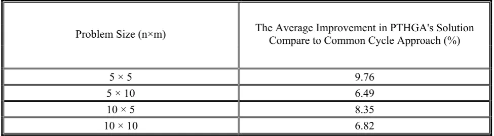
TABLE 3. Results of Medium and Large Size Test Problems (Comparison with the Common Cycle Approach).

Problem Size (n×m) The Average Improvement in PTHGA's Solution Compare to Common Cycle Approach (%)

5 × 5 9.76

5 × 10 6.49

10 × 5 8.35

10 × 10 6.82

Table 1 represents the computational results for the small sized problem instances and Table 2 and 3

In summary, we find out the following results from our numerical experiments:

• In Table 1, solution qualities of the proposed algorithm have been compared with the related optimal solution obtained via LINGO 6.0. As we can see, for the small size problem instances, the solutions of the PT-HGA are 67 times better than the solutions of LINGO. It seems that having a mixed zero-one and nonlinear nature of the proposed mathematical model makes the LINGO can not obtain good results. Also, in average, the solutions qualities obtained by the PT-HGA are 4.3 percent better than the solutions of LINGO. Totally, the results shown in Table 1 indicate superiority of the proposed algorithm with respect to both CPU time and solution quality in compare to solutions of the LINGO.

• For the medium and large-sized problem instances, performance ratio λ has been calculated and used as a measure to evaluate the proposed algorithms. In Table 2, we have calculated the performance of the proposed algorithm. We observe that the average performance ratio for the problem instances increases when the problem size increases. However, this increase can be either due to an increase in the difference between the lower bound and the corresponding optimal cost, or due to reduction of effectiveness (performance) of the proposed algorithms due to increase in corresponding solution space.

• Table 3 reports the average cost differences between the solutions obtained through proposed algorithm and the solutions of common cycle approach. These results reveal the average improvement of 7.85 percent in solutions of the PT-HGA over the common cycle's solutions, respectively. Totally, these results indicate superiority of applying the basic period policy versus common cycle approach in the problem.

7. CONCLUSION REMARKS

In this paper, the basic period approach has been

applied to solve the economic lot and delivery-scheduling problem in flexible flow lines over a finite planning horizon. To do so, a new mixed zero-one nonlinear model has been developed to optimaly solve the problem. Providing an optimal solution is not a practical approach for routine decision-making in case of the medium and large-sized problems. Thus, an efficient meta-heuristic (PT-HGA) based on power-of-two policy, of basic period approach has been developed.

Since there is no other solution method for the problem, we have compared the solutions of PT-HGA with the LINGO solution software in small-sized problems. Also, for medium and large-small-sized problems, we have calculated an index λ which calculates the distance of solutions obtained by PT-HGA from a lower bound. Computational results are very promising and indicate the superiority of PT-HGA over the common cycle approach with respect to the solution quality.

8. ACKNOWLEDGEMENT

This study was supported by the University of Tehran under the research grant No. 8109920/1/01. The authors are grateful for this financial support.

9. REFERENCES

1. Torabi, S. A., Karimi, B. and Fatemi Ghomi, S. M. T.,

“The Common Cycle Economic Lot Scheduling in Flexible Job Shops: The Finite Horizon Case”, International Journal of Production Economics, Vol. 97, (2005), 52-65.

2. Ouenniche, J. and Boctor, F. F., “Sequencing, Lot

Sizing and Scheduling of Several Components in Job Shops: The Common Cycle Approach”, International Journal of Production Research, Vol. 36, (1998), 1125-1140.

3. Ouenniche, J., Boctor, F. F. and Martel, A., “The Impact of Sequencing Decisions on Multi-Item Lot Sizing and Scheduling in flow Shops”, International Journal of Production Research, Vol. 37, (1999), 2253-2270.

4. Fatemi Ghomi, S. M. T. and Torabi, S. A., “Extension

of Common Cycle Lot Size Scheduling for Multi-Product, Multi-Stage Arborscent Flow-Shop Environment”, Iranian Journal of Science and Technology, Transaction B, Vol. 26, No. B1, (2002), 55-68.

5. Torabi, S. A., Fatemi Ghomi, S. M. T. and Karimi, B.,

Chains”, European Journal of Operational Research, Vol. 173, (2006), 173-189.

6. Yang, P. C. and Wee, H. M., “A Single-Vendor and

Multiple-Buyers Production-Inventory Policy for a Deteriorating Item”, European Journal of Operational

Research, Vol. 143, (2002), 570-581.

7. Chung, C. J. and Wee, H. M., “Optimal Replenishment

Policy for an Integrated Supplier-Buyer Deteriorating Inventory Model Considering Multiple JIT Delivery and Other Cost Functions”, Asia Pacific Journal of Operations Research, Vol. 24, (2007), 125-145.

8. Yang, P. C., Wee, H. M. and Yang, H. J., “Global

Optimal Policy for Vendor-Buyer Integrated System with Just in Time Environment”, Journal of Global Optimization, Vol. 37, (2007), 505-511.

9. Wee, H. M. and Yang, P. C., “A Mutual Beneficial

Pricing Strategy of an Integrated Vendor-Buyers Inventory System”, International Journal of Advanced Manufacturing Technology, Vol. 34, (2007), 179-187.

10. Hahm, J. and Yano C. A., “The Economic Lot and

Delivery-Scheduling Problem: The Common Cycle Case”, IIEE Transactions, Vol. 27, (1995a), 113-125.

11. Hahm, J. and Yano, C. A., “The Economic Lot and

Delivery Scheduling Problem: Models for Nested Schedules”, IIEE Transactions, Vol. 27, (1995b), 126-139.

12. Jensen, M. T. and Khouja, M., “An Optimal Polynomial

Time Algorithm for the Common Cycle Economic Lot and Delivery Scheduling Problem, European Journal of Operational Research, Vol. 156, (2004), 305-311.

13. Bomberger, E. E., “A Dynamic Programming Approach

to the Lot Size Scheduling Problem”, Management Science, Vol. 12, (1966), 778-784.

14. Elmaghraby, S. E., “The Economic Lot Scheduling

Problem: Review and Extensions”, Management Science, Vol. 24, (1978), 587-598.

15. Yao, M. J. and Elmaghraby, S. E., “On the Economic

Lot Scheduling Problem under Power-of-Two Policy”, Computers and Mathematics with Applications, Vol. 41, (2001), 1379-1393.

16. Ouenniche, J. and Boctor, F. F., “The Multi-Product,

Economic Lot-Sizing Problem in flow Shops: The Powers-of-Two Heuristic”, Computers and Operations Research, Vol. 28, (2001a), 1165-1182.

17. Ouenniche, J. and Boctor, F. F., “The Two-Group

Heuristic to Solve the Multi-Product, Economic Lot-Sizing and Scheduling Problem in flow Shops”, European Journal of Operational Research, Vol. 129, (2001b), 539-554.

18. Ouenniche, J. and Boctor, F. F., “The G-Group

Heuristic to Solve the Multi-Product, Sequencing, Lot-Sizing and Scheduling Problem in Flow Shops”, International Journal of Production Research, Vol. 39, (2001c), 89-98.

19. Ouenniche, J. and Bertrand, J. W. M., “The Finite

Horizon Economic Lot Sizing Problem in Job Shops: The Multiple Cycle Approach”, International Journal of Production Economics, Vol. 74, (2001), 49-61.

20. Cheng, R. and Gen, M., “Parallel Machine Scheduling