ABSTRAC
According to the temperature distribution of water injection well-bore in highly deviated wells under different conditions and unstable temperature field heat conduction principles, a true three-dimensional model was established to analyze the law of variation on temperature of highly deviated wells during the water injection process, and to analyze the factors that influence the water injection well-bore in highly deviated wells; this can improve the computational accuracy of the transformation of water injection string made by the temperature, and help us predicate the transformation of water injection string more accurately during the production pro-cess. The results show that the temperature distribution of highly deviated wells are greatly affected by water injection inlet temperature or injection of water inlet temperature, water injection rate, and water injection time. With the temperature field model of highly deviated wells made in this paper, the construction quality and oil production can be highly improved by reasonably controlling the temperature. All the findings which have been obtained form a theoretical basis and the experimental research for the development of mechanical analysis simulation software have been used to calculate temperature distribution and variation of water injec-tion string in highly-deviated wells and have a great theoretical significance and practical value.
Keywords: Highly Deviated Well, Water Injection, Temperature Profile, Numerical Calculation, Experimental Research Liu Jun1, 2*, Wang Wei1, Zhang Jianzhong3, and Xiao Guohua3
1School of Civil Engineering and Architecture, Southwest Petroleum University, Chengdu 610500, China
2 Modern Design and Simulation Lab for Oil and Gas Equipment, Southwest Petroleum University, Chengdu 610500, ..China
3Drilling Technology Research Institute of Jidong Oil Field Company, Hebei, 063000, China
A Numerical Simulation Study on Wellbore Temperature Field of Water
Injection in Highly Deviated Wells
INTRODUCTION
Currently, oil exploration and development in China are facing high pressure and high temperature environment, and simultaneously many development blocks are far from artificial islands and Jacket well location, so tilt angle and displacement are growing in wells.
This type of oil is buried deeply, and well tilt angle and wellbore temperature change a lot. When string movement is restricted, a large temperature difference will result in stress and the deformation of large string changes, and then the safety of pipe string is affected [1]. Meanwhile, the formation fracture *Corresponding author
Liu Jun
Email: [email protected] Tel: +13 438019245 Fax: +13 438019245
Articale history
Received: June 09, 2015
Received in revised form: October 31, 2015 Accepted: February 20, 2016
pressure of reservoir can be easily affected by temperature [2], and the changing of wellbore temperature can easily lead to wellbore instability [3, 4]. Besides, the continuous injection of cold water into the formation makes temperature drop around bottom formation, and then produces the oil within the reservoir; thus the water viscosity changes, which will affect the oil displacement effect of water [5, 6]. Therefore, it is very significant that wellbore temperature field of water injection in highly deviated wells is accurately calculated. The true three-dimensional model is established to analyze the highly deviated well water injection process temperature variation and the influential factors of wellbore temperature field by unstable temperature field heat conduction principles herein so that the value of accurate temperature changes of the water injection in different working conditions could be calculated and the influential factors of wellbore temperature distribution could be analyzed. This research also provides valid data for the further analyses of temperature effect on the mechanical behavior caused by the temperature of the water injection string. Moreover, this research serves as a theoretical guidance for rational regulation of wellbore temperature.
THEORETICAL MODEL
Fundamental Assumptions
According to the actual situation of highly deviated wells injection wellbore temperature field, the following assumptions are put forward based on the numerical simulation models:
• Wellbore continuously and rigidly contact with pipe string, and the rigidity of pipe string is considered.
• The axis of pipe string is in accordance with the borehole axis.
• The hole trajectory of highly deviated wells is described by the Frenet formula [7].
• The computational element of the pipe string is a circular arc in the space on the inclined plane.
• Before water injection, the thermals status of the pipe string, fluid in the wellbore, and the ground are equal and in equilibrium situation. Simultaneously, the initial temperature distribution obeys a stable geothermal gradient change.
• After water injection, heat transfer is considered in the direction of wellbore radius and along the vertical depth; besides, during water injection, putting the original fluid in the wellbore extrusion of mass transfer causes heat conduction to be taken into account.
• When the wellbore temperature fields are discretized in the spatial domain, the properties of matters in each micro body domain such as heat transfer coefficient and specific heat are relatively stable.
• Water injection rate, water injection temperature, all the year round average temperature under the ground, and geothermal gradient are constant.
• Away from the wellbore axis enough in the distance of r≥Rmax, formation temperature is original ground temperature.
• Under the surface of the earth Z=Zm, temperature
Tm does not change over time; under the surface of the earth Z>Zm, original formation temperature satisfies the linear relationship of Tdz=Tm+αz,
where α is the formation temperature gradient.
Establish Model
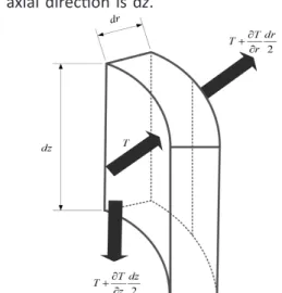
On the basis of the above assumptions, in order to the first law of thermodynamics, and the basic principles of heat transfer, the liquid in the tubing string, the string wall, liquid in the annulus, and stratigraphic unit were taken as the control volume in order to derive these control bodies energy balance equation and the mathematical model of temperature field. As shown in Figure 1, any infinitesimal bodies were taken as the control volume in the wellbore-stratigraphic system, and it was assumed that the radial distance is dr, and the borehole distance along the axial direction is dz.
Figure 1: A schematic diagram of micro element body.
The micro unit center temperature is set as T,
which, by Fourier heat conduction law, can be learned; at the place of z-dz/2 the temperature is T-(∂T/∂z)(dz/2); at the place of r+dz/2 the temperature is T+(∂T/∂z)(dz/2); at the place of
r-dz/2 the temperature is T-(∂T/∂r)(dz/2); at the place of r+dr/2, the temperature is T+(∂T/∂r)(dz/2). For example, taking a unit of the pipe string is to establish a thermodynamic equilibrium equation. The thickness of a micro unit in the column is dz, and the radial distance is equal to the string
inside radius rti. According to the assumptions, if the changes in fluid potential and fluid density were not considered, the heat of the micro element body carried over by the injected fluid from the top of wellbore per unit time may be written as follows:
2
1 f f ti f f T dzf 2
Q c r v T
z
ρ π ∂
= −
∂
(1)
The heat of the micro element body carried over by the injected fluid from the bottom of wellbore per unit time may be written as given by:
2
2 f f ti f f T dzf 2
Q c r v T
z
ρ π ∂
= +
∂
(2)
Respecting the convective heat transfer between fluid and pipe wall, and according to the Newton’s law of convective heat transfer formula, the heat of the micro element body carried over from pipe wall per unit time can be given by
(3)
The heat of the micro element body carried over by friction per unit time reads:
3
4 14 f f ti f
Q =
πλ ρ
dzr v (4)2
5 f f ti f
T
Q c r dz
t
ρ π ∂
=
∂ (5)
Heat energy variation per unit time in a micro element body can be defined as follows:
1 2 3 4 5
Q Q Q Q− + + =Q (6) Using the heat balance principles, Equation 6 can be rewritten as follows:
2 2 3 2 2 2 2 2 2 1 4 f f f ti f
f
f f ti f f tf ti
t to ti f ti
t f
f f f ti f f ti
T dz c r v T
z T dz
c r v T r dz
z
T r r T r
T T
r r
T dzr v c r dz
t
ρ π
ρ π α π
πλ ρ ρ π
∂ − − ∂ ∂ + + ⋅ ∂ ∂ − ∂ ⋅ − − − ∂ ∂ ∂ + = ∂ (7)
3 tf 2 ti t T r rt to2 ti f Tf r2ti
Q r dz T T
r r
α π ∂ − ∂
= ⋅ − − −
∂ ∂
The thermal equilibrium given in Equation 7 can be transformed into the following form:
(8)
On the basis of the same principle, the heat balance equation of the other units can be established; the true three dimensional mathematical model of temperature field for wellbore-stratigraphic system can be defined as given below.
( ) ( )
(
)
( )( )(
)
( )( )(
)
( )( ) 3 22 2 2 2 2
2
2 2 2 2 2
2 2 1 4 2 4 4 4 f f
f f ti f tf t f f f f f f
ti ti
t ti to t
t tf t f t a t t t
to ti to ti to ti
a to ci a
a t a t a c a a a
ci to to ti ci to ci to
c
T T
c r v T T v c
z r r t
T r r T
k T T k T T c
t
z r r r r r r
T r r T
k k T T k T T c
t
z r r r r r r r r
T k
ρ α λ ρ ρ
α ρ ρ ∂ ∂ − + − + = ∂ ∂ ∂ − − + − = ∂ ∂ ∂ − − − ∂ − − + − = ∂ ∂ ∂ − − − − ∂
(
)
( )( )(
)
( )( )(
)
( )( )(
)
( )( )2 2 2 2 2
2
2 2 2 2 2
2 2
2 2
4 4
4 4
1
c ci co c
a c a c e c c c
co ci ci to co ci co ci
e co ce e
e c e c e w e e e
ce co co ci ce co ce co
w w w w w w
w
r r T
k T T k T T c
t
z r r r r r r r r
T r r T
k k T T k T T c
t
z r r r r r r r r
T T T c T
r r k t
z r ρ ρ ρ ∂ − − + − = ∂ − − − − ∂ ∂ − − + − = ∂ ∂ ∂ − − − − ∂ ∂ ∂ ∂ + + = ∂ ∂ ∂ ∂ (9)
where, Cf (J/(kg°C)) is the specific heat of the fluid in the tubing string; ∂tf (W/(m2°C)) is the coefficient of
convective heat transfer between fluid in the string and pipe wall; λf is the friction coefficient of the fluid in the string, which is related to fluid Reynolds number and flow pattern; ρf (kg/m3) represents fluid
density in the string; νf (m/s) stands for the speed of the fluid motion. kt , ka , kc , ke , and kware respectively the heat conductivity coefficient of injected fluid, cylinder wall, within the annulus fluid, formation rock, injection, and the original liquid mixing unit; Similarly, ct , ca , cc , ce , and cw are respectively their specific heat capacity in J/(kg°C); ρt, ρa , ρc , ρe , and
ρw are respectively their the density in kg/m3; r
to ,
rco , rci , rti , and rce(m) are respectively the radius of the outer wall of pipe string, the radius of the outer wall of the casing, the string inner radius, the radius of the inner wall of the casing, and the cement ring diameter.
Boundary Conditions
When the wellbore temperature field model is established, boundary conditions are established as follows:
Tm is the temperature in somewhere under local annual average surface, and in general, it is a fixed value at the depth of 20 meters. Since the wellbore is axisymmetric, in the center of the hole diameter (∂T/∂r)r=0=0. Besides, since infinity away from the center line of the hole diameter, Tr=Rmax=Tdz. The adiabatic boundary for bottom hole formation is (∂T/∂z)z=l=0. The temperature of the fluid injected into from wellhead tubing or the annulus is constant; back to the exit of the boundary for the liquid temperature, (∂T/∂z)z=0=0 [8].
Initial Conditions
According to the research condition in this paper, the initial conditions are established as follows:
When t=0, the temperature of wellbore and formation is the known formation temperature distribution. Since the recovery operation is carried out continuously during each process, the next working procedure of the initial temperature condition is one end of the previous process temperature conditions.
Working Condition
When water injection process temperature field was calculated, the heat conduction caused by mass transfer during fluid injection from wellhead and the original fluid in the wellbore, which is squeezed out, must be taken into account. U (m³/min) is the volume of injected fluid flow from wellhead. Since the injected fluid is liquid, the volume is always constant and equal to U. The velocity of fluid at the cross-section Az of the fluid flow path along longitudinal Z can be written as:
( ) 3
2 1
4
f
f f ti f tf t f f f f
ti ti
f f f
T
c r v T T v
z r r
T c
t
ρ α λ ρ
(10)
There are an Lm number of Azi in the well depth of L
(i=1, 2, …, LN), and then the total time tLof injected fluid flow to the bottom of a well is worked out by:
(11)
Several typical working conditions are considered as follows:
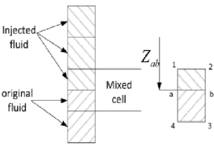
Condition one: when time is t≤tk, there are a number of interfaces of Z=Zab in the flow path. At the well depth of Z<Zab, the fluid is the injected fluid, meanwhile when Z>Zab, the original fluid is in the wellbore. Zab can be worked out by t, tk, and µz.
Therefore, a unit with two media mixing is appeared on space domain and satisfies the following heat balance equation:
(12)
Units below the well depth of Z<Zab and Z>Zab are
the same fluid, which satisfies the following heat balance equation:
(13)
Condition two: when time is t>tk, there are no mixed units, and then the heat can be calculated by Equation 1. Condition three: when the fluid in the oil tube and oil casing is static and stagnant, there are several dielectric interfaces in the flowing path and more than two kinds of medium mixing unit in spatial domain as shown in Figure 2. The actual distribution and heat transfer near the interface of two kinds of different medium within the cell are extremely complex, but all can be solved by the heat balance Equation 2 and Equation 3.
Figure 2: Fluid mixing units.
Solution Method for Model
The spatial domain is discrete by high precision of isoparametric elements adopted in this paper, and an optional implicit finite difference time domain of variable step is used in loop iteration, which obviously improves the accuracy and effectiveness of the calculation of the whole temperature field [9,10]. Next, the established temperature field model is solved by FORTRAN language programming, which is used to analyze the effect of different factors on the wellbore temperature distribution.
Factors Influencing the Temperature
of Highly Deviated Well Water Injection
Wellbore
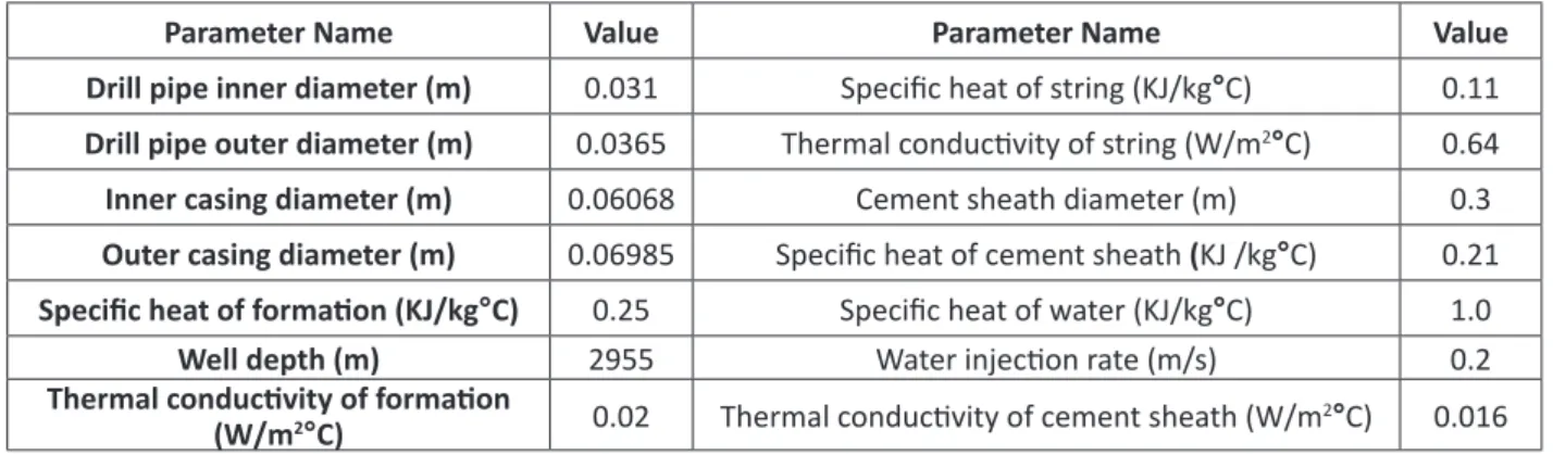
As an example, the parameters of a high angle well showed in Tables 1 and 2 are used to analyze the law of wellbore temperature field distribution with the various influential factors [11]. The controllable factors in the process of water injection included a water injection rate, water inlet temperature, water injection time, etc. In addition, wellbore temperature will also be affected by environmental factors and the structure of the borehole, etc.
0 12 1 1 34 0 1 1
0 0 1 1 1 1
( ) ( ) ( )
( / ) ( / )
o So S
o vo v
c UT c UT T n T n
V c T t V c T t
ρ ρ λ λ
ρ ρ
− − ∂ − ∂ − ∂ − ∂
= ∂ ∂ + ∂ ∂
12 34
(
)
( / )
( / )
i i I S i i i V
Table 1: Parameters of highly deviated well.
Table 2: Parameters of wellbore trajectory.
Impact of Injection Water Inlet
Temperature on the Temperature
Distribution of Highly Deviated Wellbores
The inlet temperature of water is a very important factor in oil field development. Under the conditions of a depth of 2955.7 m, a water injection rate of 0.15 m3/min, and a water injection time of 120 min,
adjusting different water inlet temperature and the chart about wellbore temperature change law of the highly deviated well are displayed in Figure 3. When the inlet temperature of water varies from 15 to 40°C, the bottom hole temperature increases by about 10°C. That is, improving the wellhead injection water temperature is equivalent to increasing more energy entering the wellbore by the pump, which increases the temperature of bottom hole. The amplitude of the increase in bottom hole temperature is associated with an increased range of
inlet temperature of the water injection; however, the temperature distribution of wellbore is not obviously affected by the water inlet temperature.
Well depth (m) Deviation angle (°) Azimuth (°) Well depth (m) Deviation Angle (°) Azimuth (°)
0 0 82.08 1673.88 4.85 301.27
231.47 0.69 40.48 1962.03 0.85 328.45
521.99 1.26 246.32 2260.76 2.41 23.14
810.03 0.83 277.98 2548.93 2.32 160.57
1097.78 11.28 301.58 2819.09 0.72 143.98
1385.81 15.24 298.55 2955.7 0.13 269.33
Impact of Water Injection Rate on the
Temperature Distribution of Highly
Deviated Wellbores
Water injection rate plays an important role in oil field development [12]; under the conditions of a
Figure 3: Wellbore temperature profiles and water temperature curve.
Parameter Name Value Parameter Name Value
Drill pipe inner diameter (m) 0.031 Specific heat of string (KJ/kg°C) 0.11 Drill pipe outer diameter (m) 0.0365 Thermal conductivity of string (W/m2°C) 0.64 Inner casing diameter (m) 0.06068 Cement sheathdiameter (m) 0.3 Outer casing diameter (m) 0.06985 Specific heat of cement sheath (KJ /kg°C) 0.21 Specific heat of formation (KJ/kg°C) 0.25 Specific heat of water (KJ/kg°C) 1.0
Well depth (m) 2955 Water injection rate (m/s) 0.2
Thermal conductivity of formation
water injection time of 120 min and a water injection initial temperature of 15°C, water injection rate is respectively 0.05, 0.08, 0.10, and 0.12 m3/min; the
wellbore temperature profile curves are presented in Figure 4. Figure 4 shows that when the water injection rate is low, injection water and rock stratum around the wellbore have sufficient time exchanging heat; therefore, the wellbore temperature is more close to the ambient temperature than the higher water injection rate. With increasing the water injection rate, the convective heat transfers between the injected water and environment time is accordingly reduced. Eventually, the temperature of bottom wellbore is decreased.
Figure 5: Wellbore temperature profiles and water injection time curves.
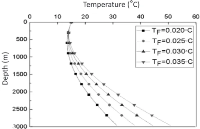
Impact of Geothermal Gradient on the
Temperature Distribution of Highly Deviated
Wellbores
Under the conditions of a water injection time of 120 min, a water injection initial temperature of 15°C, and a water injection rate of 0.1 m3/min, wellbore temperature profiles
and geothermal gradient curves are presented in Figure 6. The picture shows that with increasing geothermal gradient, wellbore temperature increased significantly. As the well becomes deeper, the temperature of the bottom hole becomes higher and higher. Hence, the precise prediction of the geothermal gradient willhave a great influence in order to predict wellbore temperature profile [13].
Impact of Water Injection Time on the
Temperature Distribution of Highly Deviated
Wellbores
Wellbore temperature is higher in a shorter injection time as shown in Figure 5. With increasing injection time, the temperature of formation around the wellbore is reduced. Also, when heat exchange between wellbore and formation tends to be stable, wellbore temperature is relatively low.
Figure 6: Wellbore temperature profiles and geothermal gradient curves.
Figure 4: Wellbore temperature profiles and water injection rate curves.
Dep
th (m)
Temperature (°C)
Dep
th (m)
Temperature (°C)
Dep
th (m)
The Experiment to Measure the Temperature
Field Distribution
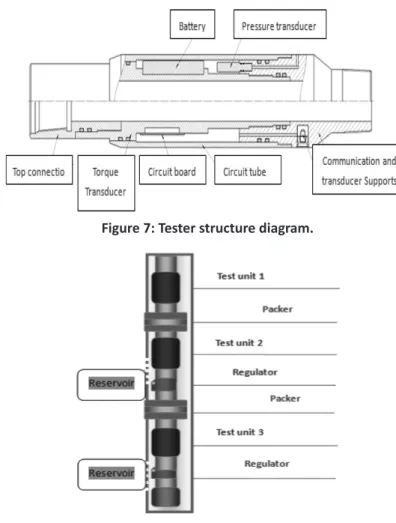
The stress measurement system of the downhole stringis composed of two parts: the downhole string stress test device and the computer data acquisition software. As shown in Figure 7, the downhole string stress test device is connected to the working string in the pipe string and to the measures.
The tester structure diagram is shown in Figure 8. The measuring device is built in a single-chip controlled manner by setting the sampling and external pressure, temperature, axial load, and torque data, and the data collected by the single-chip are stored in the memory. When the operation is finished, the data in the test device is transferred through dedicated communication lines to computer data software.
Figure 7: Tester structure diagram.
Figure 8: A schematic diagram of test process.
Figure 10: Comparison of the experimental and theoretical results.
CONCLUSIONS
The true three-dimensional model which has been proposed in the current paper can accurately calculate the distribution of temperature in different water injection conditions; besides, this model can provide technical support to prevent wellbore temperature [14] from becoming too high and thus producing a larger temperature stress and avoiding borehole wall collapse [15] in the process of water injection. Figure 10 shows that the results of the experiments and in good agreement with the theoretical calculations. Additionally, water inlet temperature does not obviously affect the wellbore temperature distribution except for water injection rate, water injection time, and geothermal gradient. It is necessary that the
geothermal gradient be accurately measured and then water injection rate and water injection time, in descending order, be reasonably controlled. The results are consistent with those reported in the literature [14]. Finally, the results have a great theoretical significance and practical value.
REFERENCES
1. Baoxia Q., Ceji Q., Chongchong S., and Jian S., “Analysis and Design Research for Layered Water Injection String Mechanics,” Petroleum Engineering Technology in Chinese, 2015, 1, 57-59.
2. Fan Y., Baodong Ch., Wenquan J., Yu Sh. et al., “Application Research of P-R State Equation in Thermodynamic Properties Calculation of Natural Gas,” Contemporary Chemical Industry, 2013, 42,
649-650.
3. Xiangqing H., Xiangjun L., and Pingya L., “Influence of Temperature Perturbation on Borehole Wall Stabilization and Oil Field Development,” Natural Gas Industry, 2003, 23, 39-41.
4. Yin S., Towler B. F., Dusseault M. B., and Rothenburg L., “Fully Coupled THMC Modeling of Wellbore Stability with Thermal and Solute Convection Considered,” Transport in Porous Media, 2010, 84, 773-798.
5. Xuefeng J. and Weige J, “Temperature’s Impact on High Pour-Point Oil Reservoir Development Effect,”
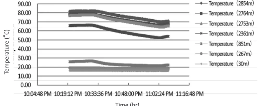
Figure 9: The temperature of different depths and injection water times.
Temperature (°C)
Dep
th (m)
Temper
atur
e (
°
C)
Journal of Gui Zhou University of Technology (Natural Science Edition), 2009, 37, 9-11.
6. Shaddel S., Hemmati M., Zamanian E., and Nejati Moharrami N., “Core Flood Studies to Evaluate Efficiency of Oil Recovery by Low Salinity Water Flooding as A Secondary Recovery Process,” Journal of Petroleum Science and Technology, 2013, 3, 65-76. 7. Xingbo W., Xixiang Ch., Limie L., “Frenet Formula
of Arbitrary Parameter,” Journal of Hunan Institute of Technology,2005, 2, 1-4.
8. Ning W., Bao Jiang S., and Zhi Yuan W., “Boundary Condition Handling for Analytical Calculations of Circulating Mud Temperatures,” Proceedings of Thirteenth National Conference on Water Dynamics and the Twenty-Sixth National Symposium on Water Dynamics, 2014, August.
9. Donea J. and Huerta A., “Finite Element Methods for Flow Problems,” 2003, John Wiley and Sons. 10. Harari, I. and Hauke, G.” Semidiscrete Formulations
for Transient Transport at Small Time Steps,”
International Journal for Numerical Methods in Fluids, 2007, 54, 731-743.
11. Aslanyan I., Barghouti J., and Al-Shammakhy
A. J., “Evaluating Injection Performance with High Precision Temperature Logging and Numerical Temperature Modeling,” SPE Reservoir Characterization and Simulation Conference and Exhibition, Society of Petroleum Engineers. 2013,
September.
12. Xiaoyan Y., Shenglai Y., Xianghong W., Jie L. et al.,
“Numerical Simulation Study on the Influence of Water Injection on the Temperature Field of High Pour Point oil Reservoir,” Complex Hydro-Carbon Reservoirs, 2011, 4, 51-53.
13. Shi Y., Song Y., and Liu H., “Numerical Simulation of downhole Temperature Distribution in Producing Oil Wells.” Applied Geophysics, 2008, 5, 340-349. 14. Wu K., Li X., Ruan M., Yu M. et al., “Dynamic
Tracking Model for the Reservoir Water Flooding of a Separated Layer Water Injection Based on a Well Temperature Log,” Journal of Petroleum Exploration and Production Technology,2015, 5, 35-43. 15. Baohua W., Xiaofeng L., and Bingyin W., “Law of
Temperature Influence on Wellbore Stability in Hot Well”. Drilling Fluid and Completion Fluid, 2004, 21,