RESEARCH NOTE
A BRANCH-AND-BOUND METHOD FOR FINDING
FLOW-PATH DESIGNING OF AGV SYSTEMS
R. Zanjirani Farahani and F. Ghasemi Tari
Department of Industrial Engineering, Sharif University of Technology Tehran, Iran, [email protected] - [email protected]
(Received: November 16, 1999 – Accepted in Revised Form: July 9, 2001)
Abstract One of the important factor in the design of automated guided vehicle systems (AGVS) is the flow path design. This paper presents a branch-and-bound algorithm to determining the flow path by consideringnot onlyloaded-vehicles, but also empty-vehicles. The objective is to find the flow path, which will minimize total travel of loaded vehicles.We know that in branch-and-bound method a branch can be fathomed in different ways, but it sometimes causes infeasible solutions. By branching on only feasible solutions, the algorithm presented in this paper works effectively. We also use DFS algorithm for finding only feasible solutions of the problem and by testing the objective function, one efficient flow path can be determined.
Key Words AGV Systems, Flow Path Design, Depth First Search
ﭼ
ﻩﺪﻴﻜ
ﻦﻳﺮﺘﻤﻬﻣﺯﺍﻲﻜﻳ ﻋ
ﺖﺳﺍﺖﻛﺮﺣﺮﻴﺴﻣ ﻲﺣﺍﺮﻃ،ﺭﺎﻛﺩﻮﺧﺮﺑﺭﺎﺑﻱﺎﻬﻤﺘﺴﻴﺳﻲﺣﺍﺮﻃﺭﺩﻞﻣﺍﻮ
.
ﺍ
ﻪﻟﺎﻘﻣﻦﻳ
ﻴﺴﻣﻦﻴﻴﻌﺗﻱﺍﺮﺑ
ﺮ ﻧﺖﻛﺮﺣ
ﻪ
ﻪﺋﺍﺭﺍﻥﺍﺮﻛﻭﻪﺧﺎﺷﺵﻭﺭﻚﻳﻲﻟﺎﺧﻞﻳﺎﺳﻭﻱﺍﺮﺑﻪﻜﻠﺑ،ﻩﺪﺷﺭﺎﺑﻞﻳﺎﺳﻭﻱﺍﺮﺑﻂﻘﻓ
ﻣ ﻲ ﻫﺩ ﺪ . ،ﻑﺪﻫ ﺎﻳ ﻓ ﻣﻦﺘ ﺴ ﻴ ﺮ ﺣ ﺮ ﻛ ﺖ ﺑ ﻪ
ﺩﻮﺷﻪﻨﻴﻤﻛ ﻩﺪﺷﻲﻃﻪﻠﺻﺎﻓ ﻞﻛﻪﻛ ﺖﺳﺍﻱﻮﺤﻧ
.
ﻲﻣ ﻴﻧﺍﺩ
ﺵﻭﺭﺭﺩﻪﻛﻢ
ﺮﻛ ﻭﻪﺧﺎﺷ ﺍ ﻥ ، ﺳﺍﻦﻜﻤﻣ
ﻻﺩ ﻪﺑﻪﺧﺎﺷ ﻚﻳﺖ
ﻪﻜﻳﺭﻮﻄﺑ ؛ﺩﻮﺷﻪﺘﺴﺑ ﻒﻠﺘﺨﻣﻞﻳ ﻜﻳ
ﻪﺑ ﻥﺪﺷﻪﺘﺴﺑ ﺎﻬﻧﺁﺯﺍ ﻲ ﺩ ﻞﻴﻟ ﻴﻏ ﻣﺮ ﻪﺟﻮ
ﺖﺳﺍﺏﺍﻮﺟﻥﺩﻮﺑ
.
ﺩ ﺭ ﺍﻳ ﻦ
ﻪﺧﺎﺷﺎﺑﻪﻟﺎﻘﻣ ﺩﺯ ﻥ ﻘﻓ ﻂ ﻭﺭ ﻱ ﻮﺟ ﺍ ﺟﻮﻣﻱﺎﻬﺑ
ﻣﻮﺤﻧﻪﺑﻢﺘﻳﺭﻮﮕﻟﺍ،ﻪ ﺛﻮ ﻱﺮ ﻛ ﺭﺎ ﻣ ﻲ ﻨﻛ ﺪ . ﻤﻫ ﭽ
ﺭﻮﮕﻟﺍﺯﺍﻪﺟﻮﻣﻱﺎﻬﺑﺍﻮﺟ ﻦﺘﻓﺎﻳﻱﺍﺮﺑﻦﻴﻨ ﻳ
ﻢﺘ ﺟ
ﻲﻣﻩﺩﺎﻔﺘﺳﺍﻖﻤﻋﻦﻴﻟﻭﺍﻱﻮﺠﺘﺴ ﻢﻴﻨﻛ
. ﺕﺭﻮﺻﻦﻳﺍﻪﺑ
ﻱﺮﺛﻮﻣﺖﻛﺮﺣﺮﻴﺴﻣ،ﻑﺪﻫﻊﺑﺎﺗﻲﺳﺭﺮﺑﺎﺑ ﺩﻮﺷﺺﺨﺸﻣ
.
INTRODUCTION
An automated guided vehicle (AGV) is a driverless vehicle used for transportation goods and materials throughout a facility, usually by following either a wire guide-path painted on the floor [1]. A system controller is responsible for the regulation of traffic when more than one vehicle is in system. One of the most important design vehicles is the guide path layout. The AGVS guide path configurations discussed in previous research include: I- conventional (Gaskin and Tanchoco [2], Kaspi and Tanchoco [3], Venkataramanan and Wilson [4]), II- tandem (Bozer and Srinivasan [5], Lin et al. [6]), III- single loop (Tanchoco and Sinriech [7], Sinriech and Tanchoco [8]), IV- bi-directional shortest path (Kim and Tanchoco [9], Chhajed et al. [10]) and V- the segmented flow topology (SFT) (Sinriech and
Tanchoco [11]). Related work in facility layout design includes Langevin et al. [12] and Banerjee and Zhou [13]. In conventional configurations, flow path is unidirectional. Unidirectional flow occurs when vehicle travel is restricted to only one direction along a given segment of the flow path. With unidirectional travel, a vehicle may have to travel a greater distance in moving from one point to another than it would if bi-directional flow is allowed. On the other hand, unidirectional flows require fewer controls and are more economical. The objective is to minimize the total distance traveled by loaded vehicles subject to the constraint that the resulting network consist of a single strongly connected component. This constraint assures that a vehicle can leave any station in the facility, visit any other station.
to be successfully utilized. There are several factors, which contribute to efficient material flow. The first is the choice of the appropriate vehicle type(s). Shelton and Jones [14] have developed a selection model that assists to user in evaluating his requirements and provides a set of AGV types that meet the user needs.
Maxwell and Muckstadt [15] addressed the issues of vehicle requirements and routing. Given a flow path, their method will simultaneously consider the minimum number of vehicles, the vehicles routs, and the number of trips over each route to meet the material handling requirements. Leung et al. [16], who allowed the capacity and speed of the vehicles to differ, extended this work.
Blair, Charnsethikul, and Vasques [17] also addressed the issue of vehicle routing. Their heuristic algorithm assumes that the number of vehicles and the flow path are given. It seeks to organize material movement into tours with the objective of minimizing the maximum tour length. Another factor that contributes to efficient material flow is dispatching. Egbelu and Tanchoco [18] presented a number of heuristic rules for dispatching AGVS and used simulation to evaluate effectiveness of these rules in different job shop environments.
All of the work mentioned thus far assumes that the flow-path design is given. Gaskin and Tanchoco [2] first proposed a method, which uses zero-one integer programming to determine the optimal, unidirectional flow path. The objective of their program was to minimize the total distance traveled by loaded vehicles. This method results in a nonlinear objective function and requires many sets of constraints. The constraint formulation requires evaluation of various shortest paths from the points of material pickup and material delivery. In a follow up paper, Kaspi and Tanchoco [3] proposed a branch-and-bound technique for solving the same problem. Venkataramanan and Wilson [4] presented an algorithm for determining the optimal, unidirectional flow path for an AGVS with a given facility layout. They formulated the problem as an integer program. The objective was to minimization the total distance traveled by vehicle subject to the constraint that the resulting network consist of a single strongly connected component and a specialized branch-and-bound solution procedure was discussed. In last three papers, the pickup/delivery stations
were assumed stationary.
The simultaneous determination of flow direction and locations of pickup/delivery stations in a given facility has also been addressed by several researchers. Goetz and Egbelu [19] presented a zero-one integer-programming model for determining the location of pickup/delivery stations based on a finite set of available sites. Riopel and Langevin [20] presented a penalty-based heuristic method for locating pickup/delivery stations. In a conceptual study, Kiran and Tansel [21] presented a strongly polynomial solution for the problem of locating a pickup point on a material handling loop network where the locations of the network-centers are fixed. In another study Kiran et al. [22] presented evidence suggesting that in solving the problem of locating stations on a unidirectional loop network, LP relaxation solutions are optimal. Kouvelis and Kim [23] later proved that assigning machines to candidate locations in a unidirectional loop network to minimize total material handling cost is NP-complete.
for the load requests, and the materials have to wait to be removed. On the other hand, when the system is always in the work center-initiated situation, there are too many vehicles in the system. As the number of vehicles in the system decreases, the impact of the vehicle- initiated dispatching rule on the waiting time for load requests increases. Although the dispatching rules used in atypical system are usually a combination of both work center- and vehicle-initiated rules [14], an ideal environment is to have as few vehicles as possible while at the same time keeping the proportion of time in which the system uses the vehicle- initiated rules as small as possible. This can be accomplished by choosing an appropriate work center- initiated dispatching rule [26].
Few researchers have used analytical methods to explore the relationships between vehicle dispatching rules and other decision variables. For example, the empty vehicle-dispatching rule developed by Srinivasan et al. [27] considers only one vehicle, which is unrealistic in real-life situations. In 1998, Kobza et al. [28] used a discrete time Markov chain based on vehicle location and represented dispatching rules in the one-step transition matrix, and considered empty vehicle travel. This paper presents an especial branch-and-bound algorithm to determine flow-path in conventional form. The objective is to find the flow path that minimizes the total travel of loaded vehicles. We use an algorithm and call it Revised- DFS algorithm, for finding only feasible solutions, because we have made it by changing DFS algorithm in graph theory.
DEFINITION OF PROBLEM
A network can easily represent the flow-path design problem [4]. For example you consider block layout of a production plant partitioned into p polygonal zones Z1, Z2, …., Zp; as illustrated in Figure 1 a block layout with 11 departments. These zones need not be convex, but they only contain 90 and 270-degree angles. Suppose you have a block layout, say output of CRAFT or any other software.
In this network, the set of vertices, denoted as V, represents corner and intersections of the given facility layout. Some of these vertices are pre-specified to be picking up (P) and delivery (D) stations and some are intersection points. The possible directions of travel
between vertices are represented by a set of edges, denoted as E (Throughout this article the word edge
will be used to indicate an undirected edge, and the word arc will be used for a directed edge).
Figure 1. Production plant partitioned into eleven level.
Figure 2. Production plant partitioned into three zones with pickup, delivery and intersection points.
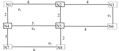
Figure 3. Production plant in Figure 2 without any difference between nodes.
Thus the facility layout can be regarded as a graph G = (V,E). For example you can suppose block layout in Figure 2, regarding to type of nodes. We define, hereafter, edges with e, nodes of graphs with N, degree 2 nodes with dotted boxes and the other nodes with filled boxes. The reason
Z10
Z8
Z11 Z9 Z7
Z3
Z6 Z4
Z1 Z2 Z5
4
4
N7
N5 N2
N8
N3
2 e5
6 2
4 N1 1 e1
3
2 e3
5
e4 N6
N4
4
4
1
2
6 D2
2
4
3
2 5
D3
will be explained.
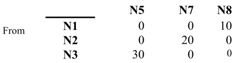
In Figure 2, the length of each edge is shown. This example can be generalized as a form with no difference between pickup and delivery stations. We knew that in From-To chart the total of picked up loads equals to the total of dropped off loads. By our definition for layout graph, consider Figure 3 as another example in which all of nodes are similar.
Now, if we consider Table 1 as a From-To chart, we will see that all types of the nodes are similar to each other, although in nature these are different.
Gaskin and Tanchoco [2] presented the general mathematical formulation of this problem. The objective function is to minimize the sum of the loaded travel. Constraints must ensure that the travel between any two adjacent vertices is unidirectional and layout graph must be strongly orientable graph.
In summary our problem is converting layout graph to a digraph in which there is at least one way between any two points in order to travel the load (in From-TO chart). In this digraph every edge must be unidirectional. We call this digraph a strongly connected digraph.
Since there is more than one way for converting a graph to strongly connected digraph, we must choose the one in which objective function be minimized. The definitions that follow are adapted from Minieka [29]: A graph G is called strongly connected if for any vertices i, j
∈
V a path from i to j exists.Up to this point, only movement of loaded vehicles have been considered. In some circumstances, the travel of empty vehicles is a secondary concern in flow-path design. In others, however, empty- and loaded- vehicle travels are equally important. Both of these cases will be considered in this section. If empty vehicles are a secondary concern, the objective function is
Min
M
L
pdS
pdL
dpR
dpp d
[
* (
*
)
*
]
,
+
∀
∑
M = preemptively large weight associated with loaded- vehicle travel ratio to empty vehicle, Lpd = number of loads shipped per unit time from
pickup station p to delivery station d (normally equal to Ldp, the number of times that empty
vehicles travel from delivery station to pickup station),
Spd = shortest path from p to d given eij’s,
Rdp = shortest path for return of empty vehicle
from d to p given eij’s.
Now, in previous example you suppose, M=3, and Lpd is transpose of elements in Table 1 as
Table 2.
DEPTH-FIRST-SEARCH (DFS)
The algorithm, which will be presented, is based on DFS method. The DFS method has designed for testing connectivity of a graph. It has developed to convert a connected and bridgeless graph to a strongly connected digraph. The algorithm is as follows [30].
Let the vertices of the graph G be
v v
1, ,...,
2v
n. Select an arbitrary vertex and labelit as 1. Pick any vertex adjacent to 1. This is not yet labeled, so label it as 2. Mark the edge {1,2} as a used edge so that it will not be used again. Proceeding similarly, suppose that we label vertex Vi with integer K. Search among all the unlabeled adjacent vertices of this vertex, select one of them and label it as (K+1). Mark the edge {K, K+1} as a used edge. Now it may be the case that all the TABLE 1. From-To chart for layout graph in Figure 3.
To
N5
N7
N8
N1
0
0
10
N2
0
20
0
N3
30
0
0TABLE 2. Transpose of From-To chart in Table 1 for Figure 3.
To
N1 N2 N3
N5
0 0 30
N7
0 20 0
N8
10 0 0
From
adjacent vertices of K are labeled. If so go, back to vertex (K-1) and search among its unlabeled adjacent vertices. If we find one such vertex, label it as (K+1) and mark the edge {K-1, K+1} as a used edge. Continue the process until all the vertices are labeled or we are back at vertex 1 with at least one vertex unlabeled. If it is not possible to label all the n vertices by the DFS technique, we conclude that the graph is not connected.
If G is connected and bridgeless, consider G is a graph model in which the vertices are the street corners of a large city. Two vertices are joined by an edge if there is a street joining them.
We are now interested in converting all streets in the city into one-way streets. Since G is strongly orientable graph every corner can be reached from every other corner after. How is this conversion carried out? We again resort to the DFS procedure and label all vertices. If {i, j} is a marked edge where i
<
j, convert this edge into an arc from i to j. On other hand, if {i, j} is an unmarked edge where i<
j, convert this edge into an arc from j to i. The resulting digraph G’ is a strong orientation of G.THE ALGORITHM
Recall that, using the DFS algorithm for making a connected digraph had three phases:
(a) Labeling all of nodes and marking some edges: we saw that in this stage, for every type of labeling we will have one spanning tree. Then, if the layout graph has n nodes, there will have n-1 marked edges. (b) Directing all of the marked edges from label with less value toward label with greater value. (c) Directing all of remaining edges from label with greater value toward label with less value. We know that above procedure creates some feasible solutions. In fact, for every situation of labeling (the nodes) and marking (the edges), we will have one feasible solution. Now, we propose Revised-DFS method. In this method, for every situation of labeling and marking, we can find more than one feasible solution, and we can find better solutions. Revised-DFS method will work in following way:
(a) Labeling all of nodes, marking the edges (similar to the Phase (a) in normal DFS).
(b) Directing all of the marked edges from label with less value toward label with greater value edges (similar to the Phase (b) in normal DFS). (c) Finding all of walks in the directed spanning tree obtained from Phase (b), from every leaf (leaf is every nodes with indegree = 1 and outdegree = 0) to the root (the root is the node labeled 1 with indegree =0 and out degree = 1).
(d) Directing all of remaining un-directed edges in every (two) possible direction.
We will prove that, every resulting digraph with above procedure will be one strongly connected digraph (feasible solution). Now, we show the procedure through one example.
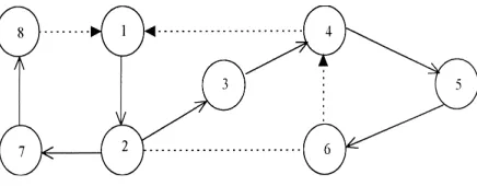
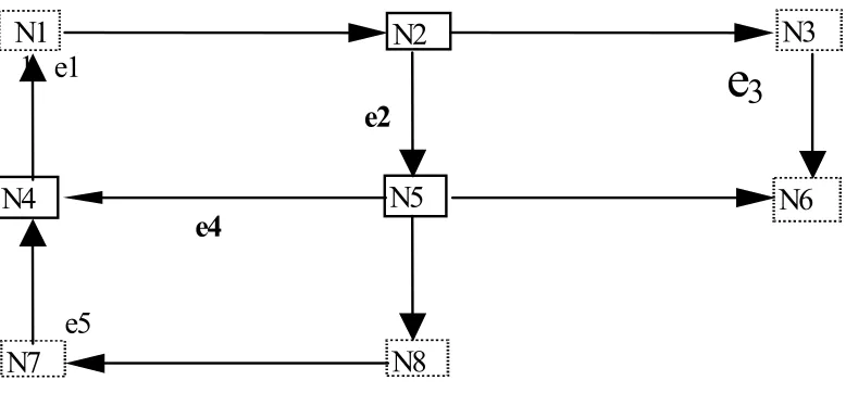
Suppose after Phases (a) and (b), we will have following directed spanning tree in Figure 4. After doing Phase (b), we know that the node 1 is root and the nodes 6 and 8 are leaves. Now, based on Phase (c), we should find every walk from 6 to 8 and from 8 to 1 (these walks cannot be opposite with the directed edges). For example, the walks 6-4-1, 6-2-3-4-1 and 6-2-7-8-1 all can be used. Suppose we use 6-4-1 for the leaf 6 and 8-1 for the leaf 8. Regarding to this, we will have Figure 4. An example of Revised-DFS after running phases a
and b.
Figure 5. Then, with respect to Phase (d), directing as 2-6 or 6-2 creates two feasible solutions. We will show that, this procedure makes only feasible solutions (but we are not sure that it covers all of feasible solutions).
Theoream
: Revised-DFS method output, results only feasible solutions.Proof:
If resulting digraph will be strongly connected, we will have a feasible solution. We must show that there is at least one walk from i to j and vice versa (for all i,j).Case 1- There is walk from 1 to every j, for every j, because of DFS nature.
Case 2- There is walk from every i to every j, if i<j and i is not a leaf, because of DFS nature.
Regarding to above case, following situations can be occurred:
Situation 1
- If i is a leaf, there is at least one walk from i to root 1 (because of Phase (c) in Revised-DFS). Now, we have walk from i to 1, and based on Case 1, there is walk from 1 to every j. Then, there is walk from i to every j (if i is a leaf).Situation 2
- If i is not a leaf, we can move from i to j (i<j) because of Case 2, as j is leaf. Now, via situation 1, we can move from j (a leaf) to every node.In summary, there is at least one walk from i to j and from j to i for every i,j.
By above procedure, we can enumerate (probably some of) feasible solutions, and we can find the best between these feasible solutions. Then, we are not sure that Revised-DFS covers all of feasible solutions, and for testing efficiency we use computer programming.
BRANCH AND BOUND APPROACH
The specific technique used in the branch and bound with depth-search first and backtracking rather than jump-tracking type of approach. Using the backtracking method a feasible complete solution (not necessarily optimal) is obtained very quickly and the required memory is much less than for jump-tracking method. The proposed approach involves eight steps. Each of these steps is described below. But first, some additional definitions are needed. {D} : the set of directed arcs
{U} : the set of undirected arcs
{A} : the set of all the arcs, i. e. {U}
∪
{D} = {A}, {U}∩
{D} =φ
UB : upper bound, i.e. the current (known) best value of the objective function. The initial value of UB is set at infinite. Any time a feasible complete solution is obtained with a value less than UB, the value of upper bound UB is updated.
LBk : lower bound of branch k is the best
value of the objective function with all arcs in
{U}. The lower bound LBk is used to label the
branches in the search process. Any time a lower bound of a certain branch is greater than (or equal to) upper bound UB, this branch is bounded.
For clarity’s, the proposed branch - and - bound method is explained through a simplified numerical example. The departmental layout, graph layout and the material flow From-To chart are given in Figure 3, and Table 1.
Step 1. Initialization
Figure 3 is the corresponding graph of the layout graph shown in Figure 2; this graph is equivalent with node-arc network in which every edge can be changed to two arcs in opposite directions. The procedure is initiated by determining set {A}. Initially, {A} = {set of all 20 arcs in Figure 3, which can be in every direction}. Since all the arcs are currently undirected {U} = {A} and {D}=φ
. The upper bound UB =∞
.Step 2. Branching
Branching process, has three stages: (I) Phases (a) and (b) of Revised-DFS. (II) Phase (c) of Revised-Revised-DFS. (III) Phase (d) of Revised-DFS.Step 3. Calculating LB
For each branch,N7
e5
N5
N2
N8
N3
N1
1
e1
N6
N4
e2
e4
e
3
we know direction of the edges in {D}. The other edges {U}={A}-{D} should be considered bi-directional. In stage k, we calculate LBk =
∑
f Y
lm lm that regarding tothese directions, is shortest path between node l and m, and flm is delivered load between l and
m (in From-To chart).
Step 4. Setting
Bounds In this algorithm there is no infeasible solution. Then branch k is bounded if: (I) lower bound LBk >upperbound UB and (II) all nodes are labeled and we have found a complete feasible solution.
Step 5. Branch Selection
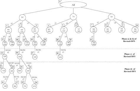
Considering the all-new branches (see the branching procedure), the one with lowest LB is selected. The information on the other branch (LB, {U}, {D}) is recorded. If both branches are bounded, the backtracking procedure (step 7) is evoked.The lower bound of branch k = 1 is LB1 =
410 and for branch k = 2, LB2 = 410, ... . Now,
in stage one, we have 10 new branches, the branches 1, 2, 3 or 5 can be selected (Figure 6). The branching process is continued with LB1 = 410.
Step 6. Updating of Upper Bound
In a branch, when all of the graph nodes are labeled, all walks are found, and all remaining undirected edges are directed, value of objective function for this feasible solution, LBk , is less than UB (the current best value ofthe objective function), then UB is updated; i.e. UB = LBk. For example, LB16 = 440 is a
feasible solution. Up to now, UB has been equal to
∞
so UB is updated to be equal to 440.Step 7. Backtracking
The backtracking procedure is invoked any time a feasible complete solution is obtained. The backtracking returns to the source branch. If a previously not selected branch of the source, i.e. a sibling branch is available (i.e. it is not bounded and it has not been selected before), then the procedure continues through this branch. Ifsibling branches are not available, then backtracking is performed again. Referring to Figure 6, the branch k =17 represents a feasible complete solution, so the procedure returns to its source, the branch k=2, the sibling branches are k=18, 19.
Step 8. Termination
When backtracking reaches the root (k =0 ), and all branches are ended or bounded (Step 4), then the search is terminated. The optimal flow path layout for the example problem (of B&B, not real problem) is shown in Figure 7.COMPUTATIONAL RESULTS
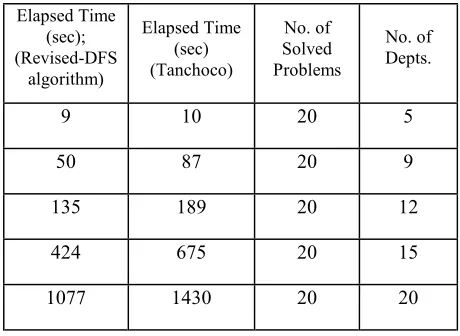
In this algorithm, we saw that every solution obtained from the algorithm is feasible, but we can’t prove that we can find all of the feasible solutions by this method. In worst case, we suppose this algorithm checks only some of feasible solutions, and branch-and-bound help us for finding the best solution between only those feasible. Then, this algorithm is a heuristic and for testing its efficiency we have solved about 100 different problems and you can see the results, in Table 3. Here, we have compared the result with the last Sinriech and
TABLE 3. Comparing the Computational Results.
Elapsed Time (sec); (Revised-DFS
algorithm)
Elapsed Time (sec) (Tanchoco)
No. of Solved Problems
No. of Depts.
Tanchoco optimal algorithm [31]. The results show that this algorithm can solve the problems in shorter time without error. Up to now, we have not found any difference between objective functions in both algorithms.
ACKNOWLEDGMENTS
The author would like to thank Professor J. M. A. Tanchoco and K. Eshghi for their remark and comment on this paper.
REFERENCES
1. Hodgson, T., King, R. and Monteith, S., “Developing Control Rules for an AGVS Using Markov Decision Processes”, Material Flow, 4(1), (1987), 85-96. 2. Gaskin, R. J. and Tanchoco, J. M. A., “Flow Path
Design for Automated Guided Vehicle System”,
International Journal of Production Research, 25(5), (1987), 667-676.
3. Kaspi, M. and Tanchoco, J. M. A., “Optimal Flow Path Design of Unidirectional AGV Systems”,
International Journal of Production Research, 28(6), (1990), 1023-1030.
4. Venkataramanan, M. A. and Wilson, K. A., “A Branch- and- Bound Algorithm for Flow Path Design of Automated Guided Vehicle Systems”, Naval Research Logistics Quarterly, 38, (1991), 431-445. 5. Bozer, Y. A. and Srinivasan, M. M., “Tandem
Configuration for Automated Guided Vehicle Systems and the Analysis of Single Vehicle Loops”,
IIE Transactions, 23(1), (1991), 72-82.
6. Lin, J. T., Chang, C. C. K. and Liu, W. C., “A Load Routing Problem in a Tandem-Configuration Automated Guided Vehicle System”, International Journal of Production Research, 32(2), (1994), 411-427.
7. Tanchoco, J. M. A. and Sinriech, D., “OSL-Optimal Single Loop Guide Paths for AGVs”, International Journal of Production Research, 30(3), (1992), 665-681.
8. Sinriech, D. and Tanchoco, J. M. A., “Solution Methods for the Mathematical Models and Single Loop AGV Systems”, International Journal of Production Research, 31(3), (1993), 705-725. 9. Kim, C. W. and Tanchoco, J. M. A., “Conflict-Free
Shortest-Time Bi-Directional AGV Routing”,
International Journal of Production Research, 29(12), (1991), 2377-2391.
10. Chhajed, D., Montreuil, B., and Lowe, T., “Flow Network Design for Manufacturing Systems Layout”,
European Journal of Operations Research, 57(2),
(1992), 145-161.
11. Sinriech, D. and Tanchoco, J. M. A., “SFT-Segmented Flow Topology”, In Material Flow System in Manufacturing, Chapter 8, Tanchoco, J. M. A., (Ed.), (London: Chapman and Hall), (1994), 200-235.
12. Langevin, A., Montreuil, B. and Riopel, D., “Spine Layout Design”, International Journal of Production Research, 32(2), (1994), 429-442. 13. Banerjee, P. and Zhou, Y., “Facilities Design
Optimization with Single Loop Material Flow Path Configuration”, International Journal of Production Research, 33(1), (1995), 183-204.
14. Shelton, D. and Jones, M. S., “A Selection Method for Automated Guided Vehicles”, Material Flow, 4, (1987), 97-107.
15. Maxwell, W. L. and Muckstadt, J. A., “Design of Automated Guided Vehicle Systems”, IIE Transactions, 14(2), (1982), 114-124.
16. Leung, L. C., Khator S. K. and Kimbler, D. L., “Assignment of AGVS with Different Vehicle Types”, Material Flow, 4, (1987), 65-72.
17. Blair, E. L., Charnsethikul, P. and Vasques, A., “Optimal Routing of Driverless Vehicles in a Flexible Material Handling System”, Material Flow, 4, (1987), 73-83.
18. Egbelu, P. J. and Tanchoco, J. M. A., “Characterization of Automatic Guided Vehicle Dispatching Rules”,
International Journal of Production Research, 22(3) (1984), 359-374.
19. Goets, W. G. and Egbelu, P. J., “Guide Path Design and Location of Load Pick-Up/Drop-Off Points for an Automated Guided Vehicle System”, International Journal of Production Research, 28(5), (1990), 927-941.
20. Riopel, D. and Langevin, A., “Optimizing the Location of Material Transfer Stations within Layout Analysis”, International Journal of Production Economics, 22(2), (1991), 169-176.
21. Kiran, A. S. and Tansel, B. C., “Optimal Pick-Up Point Location on Material Handling Networks”,
International Journal of Production Research, 27(9), (1989), 1475-1486.
22. Kiran, A. S., Unal, A. T. and Kirabati, S., “A Location Problem on a Unicyclic Network: Balanced Case”, European Journal of Operations Research, 62(1), (1992), 144-202.
23. Kouvelis, P. and Kim, M., “Unidirectional Loop Network Problem in Automated Manufacturing Systems”, Operations Research, 40(3), (1992), pp 533-550.
24. Egbelu, P., “The Use of Non-Simulation Approaches to Estimating Vehicle Requirements in an Automated Guided Vehicle Based Transport System”, Material Flow, 4(1-2), (1987), 33-51.
25. Malmborg, C. and Shen, Y.-C., “Heuristic Dispatching Models for Multi-Vehicle Material Handling System”, Applied Mathematical Modeling, 18, (1994), 124-133.
Based Algorithm for Automated Guided Vehicle Systems”, Design. Production Planing and Control, 9, (1), (1998), 47-59.
27. Srinivasan, M., Bozer, Y. and Cho, M., “Trip-Based Material Handling System: Throughput Capacity Analysis”, IIE Transactions, 26(1), (1994), 70-89. 28. Kobaz, J. E., Shen, Y.-C. and Reasor R. J., “A
Stochastic Model of Empty Vehicle Travel Time and Load Request Service Time in Light Traffic Material Handling Systems”, IIE transactions, 30, (1998),
133-142.
29. Minieka, E., “Optimizing Algorithms for Networks and Graphs”, Marcel Dekker, Inc., New York, (1978).
30. Balakrishnan, V. K., “Discrete Mathematics”, Prentice Hall PTR, (1991).
31. Sinriech, D. and Tanchoco, J. M. A., “Intersection Graph Method for AGV Flow Path Design”,