Solving Environmental/Economic Power Dispatch Problem by a Trust Region Based Augmented Lagrangian Method

(1)

Solving Environmental/Economic Power Dispatch Problem by

a Trust Region Based Augmented Lagrangian Method

H. Mohammadian Bisheh*, A. Rahimi Kian** and M. M. Seyyed Esfahani***

Abstract: This paper proposes a Trust-Region Based Augmented Method (TRALM) to solve a combined Environmental and Economic Power Dispatch (EEPD) problem. The EEPD problem is a multi-objective problem with competing and non-commensurable objectives. The TRALM produces a set of non-dominated Pareto optimal solutions for the problem. Fuzzy set theory is employed to extract a compromise non-dominated solution. The proposed algorithm is applied to the standard IEEE 30 bus six-generator test system. Comparison of TRALM results with the various algorithms, reported in the literature shows that the solutions of the proposed algorithm are very accurate for the EEPD problem.

Keywords: Environmental and economic power dispatch, fuzzy set theory, trust-region augmented Lagrangian method.

1 Introduction1

The main objective of Economic Power Dispatch (EPD) is to minimize the operating cost, while satisfying the load demand, and all unit and system equality and inequality constraints. In addition, the increasing public awareness of the environmental protection guidelines and the passage of the Clean Air Act Amendment of 1990 have impelled the utilities to modify their design or operational strategies in order to reduce pollution and atmospheric emissions of thermal power plants [1, 2].

Several strategies have been proposed to reduce the atmospheric emissions [3, 4], some of which are:

1. Planning to reduce the power use of power plants with higher pollution rates and use the power stations with lower emission rates.

2. Installation filters on power plants to purify the pollutant gases.

3. Switching to low emission fuels from high emission ones (e.g., using natural gas instead of mazut).

4. Replacement aged and low efficient fuel-burners and generator units by high efficient ones.

The second to fourth options require installation of new equipments, and need considerable capital

Iranian Journal of Electrical & Electronic Engineering, 2012. Paper first received 11 July 2011 and in revised form 18 Jan. 2012. * The author is with the Department of Industrial Engineering of Mazandaran University of Science and Technology, Babol, Iran. ** The author is with the Department of Electrical Engineering of Tehran University, Tehran, Iran.

*** The author is with the Department of Industrial Engineering of Amirkabir University, Tehran, Iran.

E-mails: [email protected], [email protected] and [email protected].

investments, and normally are considered as long-term planning. Hence, the first option, that is planning the power dispatch in such a manner that optimizes the fuel cost objective, as well as emission cost objective, individually, and especially simultaneously, is our concern for study.

After deregulation of electricity markets, serious competition has arisen among generating companies [5-7]. In this situation, generating companies try to reduce the cost of energy, to enable them compete in the competitive electricity markets. One of the effective methods of reducing the cost of electric energy is environmental-economic power dispatch (EEPD). In recent years, the EEPD category has considerably been investigated in different ways. In [8-10], the emission was considered as a constraint with a permissible limit, and the problem was reduced to a single objective optimization problem. The problem in this method is that a compromise optimal solution cannot be found between emission and fuel costs.

In [11], a linear programming based optimization procedure was proposed in which the objectives were considered one at a time. A compromise optimal solution is impossible in this method either.

In [12], a fuzzy multi-objective optimization approach for the EEPD problem was proposed. The solutions produced by this technique were suboptimal and the algorithm did not provide a systematic framework to direct the search towards the Pareto optimal set.

Over the past decade, the EEPD problem has received much interest due to the development of a number of multi-objective search strategies. Strength

(2)

Pareto Evolutionary Algorithm (SPEA) [2], Niched Pareto Genetic Algorithm (NPGA) [13], Non-dominated Sorting Genetic Algorithm (NSGA) [14], Multi-objective Stochastic Search Technique (MOSST) [15], Fuzzy Clustering-based Particle Swarm Optimization (FCPSO) [16], Multi-objective Particle Swarm Optimization (MOPSO) [17], Epsilon Constraint (EC) approach [18], etc., constitute the pioneering multi-objective approaches that have been applied to solve the multi-objective EEPD problem.

In the above approaches, the EEPD problem were converted to a single objective problem by using a linear combination of the objectives as a weighted sum with a long range planning like switching to low emission fuels. The positive characteristic of these methods is that a set of Pareto optimal solutions can be obtained by changing the weights. In general, while there are more than one objective function in a problem, especially when these objective functions are non-commensurable or even conflicting, instead of having one optimal solution, a set of optimal solutions are of interest. The reason for the optimality of many solutions is that no one can be considered to be better than any other with respect to all the objective functions. These optimal solutions are known as Pareto optimal solutions. There are some problems associated with taking a linear combination of different objectives as a weighted sum:

1. The combined objective function may lose significance due to the incorporation of multiple non-commensurable factors into a single function. 2. The lack of sufficient information regarding the

operation conditions make it difficult for the decision maker to decide on the preferences of objective in giving the weighting factors.

The first problem can be addressed by a proper selection of the scaling factor λ and multiplying the emission objective by this factor.

To deal with the second problem, fuzzy set theory has been used to efficiently derive a candidate Pareto optimal solution for the decision maker [19]. This approach will be explained later.

2 Problem Statement

The EEPD problem is to minimize two non-commensurable and competing objective functions, fuel cost and emission, while satisfying several equality and inequality constraints [2]. The problem is generally formulated in the following subsections.

2.1 Problem Variables

The variables of the problem are the quantities of real power of committed power plants, that is, PGi ,

N

i=1,2,..., and N is the number of committed power plants in the interconnected network.

2.2 Problem Objectives

There are two objectives which are minimization of fuel cost and minimization of emission amount.

1 Minimization of fuel cost

The generators cost curves are represented by quadratic functions [1,2]. The total $/h fuel cost

) (PG

F can be expressed as

2 1

)

( i Gi i Gi

N

i i

G a b P c P

P

F =

∑

+ +

= (1)

where N is the number of generators,ai,bi, and ciare the cost coefficients of theith generator, and PGis the

real power output of the

i

_th generator. PG is the vector of real power outputs of generators which is defined as

] , ... , ,

[ G₁ G₂ G_N

G P P P

P = (2) 2 Minimization of emission amount

The total emission E(PG) in (ton/h) atmospheric pollutants such as sulphur oxides (SOX) and nitrogen

oxides (NOx) caused by the operation of fossil–fueled thermal generation can be expressed as [2]:

) exp(

) (

10 )

( 2

2 1

Gi i i

Gi i Gi i i N

i G

P

P P P

E

λ ζ

γ β α +

+ + =

−

=

∑

(3)

where αi,βi,γi,ζi and λi are coefficients of the ith

generator emission characteristics.

2.3 Problem Constraints 2.3.1 Power Balance Constraint

The total power generation must cover the total

power demandPDand the real power loss in

transmission linesPloss. Hence,

. 0

1

= − −

∑

=

loss D N

i

Gi P P

P ₍₄₎

The real power loss Ploss in Eq. (4) is represented by calculation of the AC load flow problem, which has equality constraints on real and reactive power at each bus as follows [2]:

[

cos( ) sin( )

]

1

j B

G V V P

P ij i j ij i

NB

j j i Di

Gi= +

∑

δ −δ − δ −δ

= (5)

)] cos(

) sin( [

1 j i ij

j i ij NB

j j i Di Gi

B

G V V Q Q

i

δ δ

δ δ −

+

− +

=

∑

= ₍₆₎

where NB is the number of buses; PGiand QGiare the real and reactive power generated at the ith bus

respectively, PDi and QDi are the

i

th bus load real and

(3)

reactive power, respectively,Gij and Bijare the transfer conductance and susceptance between bus iand bus j, respectively, Vi and Vj are the voltage magnitudes at bus i and bus j , respectively, δi and δj are the voltage angles at bus iand bus j, respectively.

There are several methods of solving the resulting nonlinear system of Eqs. (5) and (6) which the most popular is known as the Newton-Raphson Method. The load flow solution gives all bus voltage magnitudes and angles that can be used to calculate the transmission losses as follows:

[

2 2 2 cos( )

]

1

j i j i j i NL

k k

loss g V V VV

P =

∑

+ − δ −δ

=

(7)

where,NL is the number of transmission lines and

k

g is the conductance of the k_th line that connects bus ito bus j.

2.3.2 Generation Capacity Constraint For stable operation, the real power output of each generator is limited by lower and upper limits as follows [2]:

. ,..., 2 , 1 , max min

N i

P P

P_Gi ≤ _Gi≤ _Gi = (8)

where, min

Gi

P and max

Gi

P are the lower limit and upper

limit power outputs of

i

_thgenerator, respectively, and

Nis the number of generators.

2.3.3 Security Constraint

For secure operation, the transmission line loading

l

S is restricted by its upper limit as follows:

NL k

S

Slk lk , 1,...,

max ₌

≤ (9)

where Slk and max lk

S are respectively the transmission

loading and upper limit transmission loading of

i

_th transmission line.

It should be noted that the k_th transmission line flow connecting bus ito bus jcan be calculated as

* )

( _i _i _ij

lk V I

S = ∠

δ

(10) where, Iij is the current flow from bus i to bus j and can be calculated as

⎥ ⎥ ⎥

⎦ ⎤

⎢ ⎢ ⎢

⎣ ⎡

∠ +

∠ − ∠ ∠

=

) 2 )( (

) )( (

)

( _y

j V

y V

V V

I

i i

ij j j i i

i i

ij _δ

δ δ

δ ₍₁₁₎

where yij is the line admittance, while y is the shunt

susceptance of the line [2].

2.4 Problem Formulation

By summing up the aforementioned objectives and constraints, the problem can mathematically be formulated as a nonlinear constrained multi objective optimization problem as follows:

)] ( , ) (

[F PG E PG

Minimize (12) Subject to

0 ) (PG =

g (13)

0 )

(P_G ≤

h (14) where, g is the equality constraint representing the power balance, and h is the inequality constraint representing the power system security and the generator capacity constraints.

The power balance constraint is as follows:

B b P

B

d _Gb

k k bk

b+

∑

( δ )− =0,∀ ∈ (15)

where b and kare number of the buses (nodes) in the electric network, db is the demand at bus b, Bbk is network susceptance matrix, δk is phase angle at busk,

Gb

P is the generating unit active power at bus b, and B

is the set of all buses.

The forward and backward power system security constraints are:

NL l H

l _k

k lk

cl−

∑

( δ )≥0,∀ ∈ (16)

NL l H

l _k

k lk

cl+

∑

( δ )≥0,∀ ∈ (17)

where, l is number of the line between bus band bus

k, lcl is the capacity limit of line l, Hlkis the network transfer matrix, and NLis the set of all lines.

The generator capacity constraint is as follows:

B b P

P_Gb+ _Gb ≥ ∀ ∈

− max 0,

(18)

where, PGbmax is the maximum generation capacity at bus

b.

In order to solve OPF problem it is necessary to select one of the buses as swing (slack) bus with the following relation:

B k swk k = ∀ ∈

− δ 0, (19) where, swk is the swing bus vector.

There are two nonnegative decision variables, with the following relations:

B b

db≥0,∀ ∈ (20)

B b

PGb≥0,∀ ∈ (21)

(4)

3 Principles of Multi Objective Optimization

Generally, nonlinear constrained multi objective optimization problems can be shown as follows [20]:

obj

i x i N

f

Minimize ( ) =1,..., (22)

Subject to

ME j

x

g_j( )=0 =1,..., (23)

MI k

x

hk( )=0 =1,..., (24)

wherefi is the ith objective function, x is a decision variable vector which representing a solution, Nobj is the number of objectives, ME is the number of equality constraints, and MI is the number of inequality constraints.

As stated already, the objective functions often do not have a common scale, and normally compete with each other. For such competing objectives, instead of looking for one optimal solution, a set of optimal solutions is of interest. The reason for the interest in these several optimal solutions is the fact that no solution can be considered to be better than any other one with respect to all objective functions. These optimal solutions are known as Pareto optimal solutions.

In this situation, any two solutions x1 and x2 for a multi objective optimization problem can have one of the two following possibilities:

The first solution x1 dominates or covers the other solution. In this case x1 is called non dominated (or dominating) solution or vice versa.

In a minimization problem, a solution x1 covers or dominates x2 if and only if the following two conditions are satisfied:

) ( ) ( : } ,..., 2 , 1 { .

1 1 2

x f x f N

i∈ _obj _i ≤ _i

∀ (25) ) ( ) ( : } ,..., 2 , 1 { .

2 1 2

x f x f N

j∈ _obj _j < _j

∃

(26) The solutions that are non-dominated within the entire search space constitute the Pareto optimal set [2] and [20].

4 Trust Region Based Augmented Lagrangian Method (TRALM)

The Augmented Lagrangian Method (ALM) [21] solves a generic optimization problem

) ( minf X

X (27)

Subject to

0 ) (X =

H (28)

0 ) (X ≤

G (29) 0

≥

X (30)

By converting it into a sequence of unconstrained optimization problems with penalty terms as follows:

{

2 2

}

1 min ) ( ]) 0 , ) ( (max[ 2 1 ) ( ] [ ) ( 2 1 ) ( ) ( ) ( ) ( k j j k j k j ni j k j k T T k k X X G U U X H W X H X H X f X L μ μ λ − + + + + =

∑

= .(31)

In Eq. (31), is the number of inequality constraints, k

λ _andμk

are trial Lagrange multipliers, and k

W _and

k

U _{are penalty parameters. In the so-called “multiplier}

method”, k, k, k,

W

λ μ _and k

U _{are updated after each}

round of unconstrained optimization

1

[ ] ( )

k k k k

W H X

λ + ₌λ ₊

(32)

{

}

1

max ( ), 0

k k k k

j j U G Xj j

μ + ₌ μ ₊

(33) 1 1 1 ( ) ( ) ( ) ( )

k k k

W j j W j

k j

k k k

j j W j

W if H X H X

W

W if H X H X

β γ γ − + − ⎧ ⎫ ⎪ ⎪ = ⎨ ⎬ ≤ ⎪ ⎪ ⎩ ⎭ f (34) 1 1 1 ( ) ( ) ( ) ( )

k k k

U j j U j

k

j k k k

j j U j

U if G X G X

U

U if G X G X

β γ γ − + − ⎧ ⎫ ⎪ ⎪ = ⎨ ⎬ ≤ ⎪ ⎪ ⎩ ⎭ f (35)

where, _Xk

is the solution of Eq. (31). Convergence is achieved provided that γW f0,γUp1,βW f1, βU f1,

and the following relations are satisfied:

( k) k

XLX X ε

∇ ≤ (36)

1 _{/ (1} ₎

k k k

λ

λ + λ λ ε

∞

− + ≤ (37)

1 _{/ (1} ₎

k k k

μ

μ + μ μ ε

∞

− + ≤ (38)

In Eqs. (36-38), ε ’s are the tolerance parameters and εk

decreases to a near-zero value ε∞ as the sub-optimization k increases. Combined with a suitable unconstrained optimization algorithm, the augmented Lagrangian method can solve large-scale nonlinear constrained optimization problems very reliably and generate accurate Lagrangian multipliers.

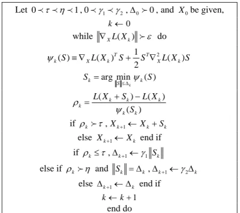
In the TRALM algorithm, we use a trust region method to solve Eq. (31). Generally trust-region methods are used to solve unconstrained optimization problems [22]. Hence the constrained problems are converted to unconstrained ones by Lagrangian multipliers and are solved by trust-region algorithms. Branch et al. proposed a two-dimensional trust-region method for solving large-scale optimization problems [23]. The pseudo code for the trust-region method adopted in TRALM is shown in Fig. 1.

5 Implementation of the Proposed Algorithm

For implementing the proposed algorithm (TRALM), the parameters have been selected as follows:

(5)

Let 0p p pτ η 1 , 0pγ1pγ Δ2, 0f0 ,and X0be given,

0

k←

while ∇XL X( k) fε do

2

1

( ) ( ) ( )

2

T T

k S XL Xk S S XL Xk S

ψ ≡ ∇ + ∇

arg min ( )

k

k k

S

S ψ S

≤Δ

=

( ) ( )

( )

k k k

k

k k

L X S L X

S

ρ

ψ

+ −

=

if ρ_kfτ,X_k+₁←X_k+S_k

else Xk+1←Xk end if

if ρk≤τ,Δk+1←γ1 Sk

else if ρ_k _fη and Sk = Δ Δk, k+₁← Δγ₂ k

else Δ_k+₁← Δ_k end if

1

k← +k end do

Fig. 1 Pseudo code for the trust-region method adopted in TRALM

33 . 0 , 3 ,

0 . 2 , 1 . 0 , 75 . 0

25 . 0 , 2 1 , 0 2 , 1 1 , 3 5

, ,

2 1

0

= =

=

= − = =

− = −

= ∞

u w u w

e e

γ β

γ γ

η

τ ε

ε ε

ε_λ _μ

Then the TRALM has been implemented in MATLAB on a Pentium 133 MHz PC and was tested on the standard IEEE 30 bus six-generator test system. The single–line diagram and the generator fuel cost and emission coefficients are shown in Fig. 2 and Tables 1 and 2, respectively [2]. The detailed data could be obtained from [2].

To compute the different Pareto optimal solutions, objective functions are linearly combined to constitute a single objective function as follows:

( G) (1 ) ( G)

Minimize wF P + −w λE P (39)

where, the scaling factor λ was selected to be 3000 in our study and wis a weighting factor [2].

As can be seen from Eq. (39), when,w=0, the single objective function calculates only the emission amount, and whenw=1, it calculates only the fuel cost. Whenwchanges from 0 to 1, for eachw, there is a Pareto optimal solution. In order to generate evenly-distributed Pareto optimal solution set,wis increased evenly by a fixed amount Δw in each step from 0 to 1. The number of wcounts the number of Pareto optimal solutions. As a matter of fact there is not a definite rule to choose the number ofw, but we generated the number of Pareto optimal sets, from 11 to 101 and computed the best compromise solutions. Comparing these best compromise solutions showed that, there is not much difference between the best compromise solutions when the number of wchanges from 21 to 101. So 21, was selected for w due to the advantage of less computation time.

Fig. 2 Single-line diagram of IEEE 30 bus test system

Table 1 Generator fuel cost coefficients Gen

No

2 G G

F= +a bP +cP $/h PGmax

Per 100 MW

min G

P

Per 100 MW

a b c

1 10 200 100 1.5 0.05

2 10 150 120 1.5 0.05

3 20 180 40 1.5 0.05

4 10 100 60 1.5 0.05

5 20 180 40 1.5 0.05

6 10 150 100 1.5 0.05

Table 2 Generator emission coefficients

Gen No

2 2

10 ( G G) exp( G)( / )

E= − α β+ P +γP +ξ λP ton h

α β γ ξ λ

1 4.091 -5.554 6.490 2.0 E-4 2.857 2 2.543 -6.047 5.638 5.0 E-4 3.333 3 4.258 -5.094 4.586 1.0 E-6 8.000 4 5.326 -3.550 3.380 2.0 E-3 2.000 5 4.258 -5.094 4.586 1.0 E-6 8.000 6 6.131 -5.551 5.151 1.0 E-5 6.667

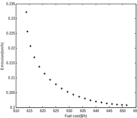
By varying w from 0 to 1 with the abovementioned procedure, the compromise solution set has been computed using TRALM, and the results are shown in Figs. 3, 4 and 5. In Fig. 3, the system is considered as lossless and the security is released (Case1). In Fig. 4,

(6)

the transmission power loss has been taken into account and the security is released (Case2). At last in Fig. 5 all three constraints have been taken into account (Case3).

600 605 610 615 620 625 630 635 640

0.19 0.195 0.2 0.205 0.21 0.215 0.22 0.225

Fuel cost($/h)

E

m

is

s

ion

(t

on/

h)

Fig. 3 The solution of TRALM approach for Case 1

605 610 615 620 625 630 635 640 645

0.19 0.195 0.2 0.205 0.21 0.215 0.22 0.225

Fuel cost($/h)

E

m

is

s

ion

(t

on

/h

)

610 615 620 625 630 635 640 645 650 655 0.2

0.205 0.21 0.215 0.22 0.225 0.23 0.235

Fuel cost($/h)

Em

is

s

io

n

(t

o

n

/h

)

6 Best Compromise Solution

Optimization of the formulated objective functions Eqs. (1) and (3) using TRALM yields not a single optimal solution, but a set of Pareto optimal solutions, in which one objective cannot be improved without sacrificing another objective. For practical applications, however, we need to select one solution, satisfying the different goals to some extent. Such a solution is called best compromise solution. One of the challenging factors for the tradeoff decision is the imprecisenature of the decision maker's judgment. For this consideration fuzzy set theory is employed [19]. The

i

_th objective value, Fi corresponding to asolution is represented by a membership function μi

⎪ ⎪ ⎩ ⎪⎪ ⎨ ⎧

≥ < < −

−

≤ =

max max min

min max

max

min

0 1

i i

i i i i i

i i

i

F F

F F F F F

F F

μ

(40)

where, Fimin is the value of an original objective

function i which is supposed to be completely satisfactory, and Fimax, is the value of the objective

function which is clearly unsatisfactory to the decision maker. For each non-dominated solution k , the normalized membership function μk is calculated as follows:

∑ ∑

∑

= = =

=

_M

k Nobj

i k i Nobj

i k i k

1 1 1

μ

(41)

where, M is the number of non-dominated solutions, and Nobj is the number of objective functions. The

function μk

in equation Eq. (41) represents a fuzzy cardinal priority ranking of the non-dominated solutions. The solution which attains the maximum membership μk in the fuzzy set can be chosen as the

best compromise solution or that having the highest cardinal priority ranking.

The values of μk_{for non-dominated solutions of the}

proposed algorithm have been calculated by a MATLAB program.

7 Results and Discussions

To demonstrate the effectiveness of the proposed algorithm TRALM, our obtained results are compared with the results obtained by the seven other algorithms reported as SPEA [2], LP [11], NPGA[13], NSGA[14], MOSST[15], FCPSO[16], and EC[18] for three Cases as follows:

(7)

7.1 Case 1

At this level the system is considered as lossless and only the capacity constraints are considered. The results obtained from the proposed algorithm on the test system, have been shown in Fig. 3.

Table 3 is provided to compare the best fuel costs of various algorithms. As can be seen from this table the fuel cost calculated by the proposed algorithm (TRALM) is less than or at least equal to the other concerned algorithms.

Table 4 has been provided to compare the best emissions of different algorithms. This table shows that the emission amount obtained from the proposed algorithm is less or at least equal to the other algorithms. It is worth to be noted that when the emission of TRALM is equal to other algorithms its fuel cost is less than the ones of the others.

Table 5 has gathered the existing best compromise solutions of the concerned algorithms. Since in compromise solution, decreasing of one objective function occurs in compensation of increasing the other one. So it is not a good measure for comparison, but Table 5 has been provided to show that the compromise solution of the proposed algorithm is quite reasonable.

The run time of TRALM, for Case1 is 11 seconds, which is greater than the run time reported in [18], and less than the one reported in [2].

7.2 Case 2

In this case the transmission losses and power balance constraints are considered, but the security constraints are released. The numerical results obtained from the proposed algorithm on the test system are shown in Fig. 4.

Table 6 is provided to compare the best fuel costs of various algorithms. This table shows that the fuel cost obtained by the proposed algorithm except in EC approach is less than the ones of the other concerned algorithms.

Table 7 has been provided to compare the best emissions of the various algorithms. It shows that the emission amount obtained from the proposed algorithm is less than or at least equal to the other algorithms. It is worth to be noted that when the emission of TRALM is equal to other algorithms its fuel cost is less than the ones of the others.

Table 8 has gathered the existing best compromise solutions of the concerned algorithms. This table represents a reasonable compromise solution for the proposed algorithm.

7.3 Case 3

In this case, all constraints including transmission losses, power balance, and security constraints are considered. The numerical results obtained from the proposed algorithm on the test system are shown in Fig. 5.

Table 9 is provided to compare the best fuel costs of the various algorithms. This table shows that the fuel cost obtained by the proposed algorithm except in EC approach is less than the ones of the other concerned algorithms.

Table 10 has been provided to compare the best emissions of the various algorithms. It shows that the emission amount obtained from the proposed algorithm except in EC approach is less than the ones of other algorithms.

Table 11 has gathered the existing best compromise solutions of the concerned algorithms. This table represents a reasonable compromise solution for the proposed algorithm.

Table 3 Comparison of best fuel costs of various algorithms for Case 1

Table 4 Comparison of best emissions of various algorithms for Case 1

LP [11] MOSST [15] FCPSO [16] NPGA [13] NSGA [14] SPEA [2] EC [18] TRALM [Proposed]

PG1 0.4000 0.4095 0.4097 0.40584 0.4072 0.4240 0.4060 0.4054

PG2 0.4500 0.4626 0.4550 0.45915 0.4538 0.4577 0.4590 0.4592

PG3 0.5500 0.5426 0.5363 0.53797 0.4888 0.5301 0.5379 0.5382

PG4 0.4000 0.3884 0.3842 0.38300 0.4302 0.3721 0.3830 0.3832

PG5 0.5500 0.5427 0.5348 0.53791 0.5836 0.5311 0.5380 0.5382

PG6 0.5000 0.5142 0.5140 0.51012 0.4707 0.5190 0.5100 0.5099

Emission (ton/h)

0.19423 0.19418 0.1942 0.1943 0.1946 0.1942 0.1942 0.1942

Cost ($/h) 639.600 644.1118 638.3577 636.04 633.83 640.42 638.2703 638.2387

PG1 0.1500 0.1097 0.1070 0.1116 0.1038 0.1009 0.1097 0.1097

PG2 0.3000 0.2998 0.2897 0.3153 0.3228 0.3186 0.2998 0.2998

PG3 0.5500 0.5243 0.5250 0.5419 0.5123 0.5400 0.5243 0.5243

PG4 1.0500 1.0162 1.0150 1.0415 1.0387 0.9903 1.0162 1.0162

PG5 0.4600 0.5243 0.5300 0.4726 0.5324 0.5336 0.5243 0.5243

PG6 0.3500 0.3597 0.3673 0.3512 0.3241 0.3507 0.3597 0.3597

Cost ($/h) 606.314 605.8890 600.1315 600.31 600.34 600.22 600.1114 600.1114

0.2233 0.2222 0.2223 0.2238 0.2241 0.2223 0.2221 0.2222

(8)

Table 5 Comparison of best compromise solutions of various algorithms for Case 1

LP [11] MOSST [15] FCPSO [16] NPGA [13] NSGA [14] SPEA [2] EC [18] TRALM

[Proposed]

PG1

Compromi se solution

was not considered

in the paper

Compromise solution was

not calculated

in details

Compromis e solution was not considered in the paper

0.2663 0.2252 0.2623 Comprom ise solution was not calculated

in details

0.2502

PG2 0.3700 0.3622 0.3765 0.3700

PG3 0.5222 0.5222 0.5428 0.5394

PG4 0.7202 0.7660 0.6838 0.7080

PG5 0.5256 0.5397 0.5381 0.5394

PG6 0.4296 0.4187 0.4305 0.4296

Cost($/h) 621.7582 608.90 606.03 610.2977 610.9634 608.8234

0.1968 0.2015 0.2041 0.2005 0.2000 0.2015

L [11] MOSST [15] FCPSO [16] NPGA [13] NSGA [14] SPEA [2] EC [18] TRALM [Proposed]

PG1

Case2 was not considered in the paper

0.1130 0.1425 0.1447 0.1279 0.1076 0.1129

PG2 0.3145 0.2693 0.3066 0.3163 0.3012 0.3024

PG3 0.5826 0.5908 0.5493 0.5803 0.5970 0.5322

PG4 0.9860 0.9944 0.9894 0.9580 0.9897 1.0215

PG5 0.5264 0.5315 0.5244 0.5258 0.5120 0.5322

PG6 0.3450 0.3392 0.3542 0.3589 0.3511 0.3629

Cost($/h) 607.7862 608.06 607.98 607.86 605.8363 606.8015

0.2201 0.2207 0.2191 0.2176 0.2208 0.2222

PG1

Case 2 was not considered in the paper

0.4063 0.4064 0.3929 0.4145 0.4102 0.4061

PG2 0.4586 0.4876 0.3937 0.4450 0.4633 0.4611

PG3 0.5510 0.5251 0.5818 0.5799 0.5447 0.5438

PG4 0.4084 0.4085 0.4316 0.3847 0.3921 0.3966

PG5 0.5432 0.5386 0.5445 0.5384 0.5447 0.5438

PG6 0.4942 0.4992 0.5192 0.5051 0.5152 0.5126

0.1942 0.1943 0.1947 0.1943 0.1942 0.1942

Cost($/h) 642.8964 644.23 638.98 644.77 646.2203 644.0792

PG1

Compromi se solution

were not considered

in the paper

Compromis e solution

were not considered in the paper

for Case 2

Compromis e solution were not considered in the paper

0.2976 0.2935 0.2752 Compromis e solution

were not considered in the paper

for Case 2

0.2694

PG2 0.3956 0.3645 0.3752 0.3817

PG3 0.5673 0.5833 0.5796 0.5463

PG4 0.6928 0.6763 0.6770 0.6815

PG5 0.5201 0.5383 0.5283 0.5463

PG6 0.3904 0.4076 0.4282 0.4388

Cost($/h) 617.79 617.80 617.57 617.5106

0.2004 0.2002 0.2001 0.2001

LP [11] MOSST [15] FCPSO [16] NPGA [13] NSGA[ 14] SPEA [2] EC [18] TRALM [Proposed]

PG1

0.1596 0.1127 0.1358 0.1319 0.2183 0.1648

PG2 0.3535 0.3747 0.3151 0.3654 0.3554 0.3456

PG3 0.7974 0.8057 0.8418 0.7791 0.5776 0.6619

PG4 0.9719 0.9031 1.0431 0.9282 0.7590 1.1079

PG5 0.08624 0.1347 0.0631 0.1308 0.5393 0.1691

PG6 0.49609 0.5331 0.4664 0.5292 0.4080 0.4147

Cost($/h) 620.18 620.46 620.87 619.60 611.2198 613.9360

0.2283 0.2243 0.2368 0.2244 0.2043 0.2322

(9)

PG1

Case 2 was not considered in the paper

0.47969 0.4753 0.4403 0.4419 0.4122 0.4649

PG2 0.5287 0.5162 0.4940 0.4598 0.4667 0.5164

PG3 0.67116 0.6513 0.7509 0.6944 0.5514 0.6201

PG4 0.5318 0.4363 0.5060 0.4616 0.4059 0.4764

PG5 0.1257 0.1896 0.1375 0.1952 0.5731 0.2091

PG6 0.5299 0.5988 0.55364 0.6131 0.4550 0.5771

0.2047 0.2017 0.2084 0.2019 0.1944 0.2008

Cost($/h) 651.62 657.57 649.24 651.71 642.70 651.5708

LP [11] MOSST [15] FCPSO [16] NPGA

[13]

NSGA [14]

SPEA [2]

EC [18] TRALM

[Proposed]

PG1

not considered in the paper for Case3

not considered in the paper for Case 3

0.2998 0.2712 0.3052 Compromise solution was

0.3126

PG2 0.4325 0.3670 0.4389 0.4262

PG3 0.7242 0.8099 0.7163 0.6508

PG4 0.6852 0.7550 0.6978 0.7994

PG5 0.1560 0.1357 0.1552 0.1809

PG6 0.5561 0.5239 0.5507 0.4941

Cost ($/h)

630.06 625.71 629.59 622.7865

0.2079 0.2136 0.2079 0.2094

8 Conclusions

Most papers reported in the literature review, used evolutionary algorithms to solve multi-objective environmental-economic power dispatch problem. The trust region based augmented Lagrangian method (TRALM) is a known and powerful technique for solving constrained nonlinear programming problems. Therefore in this paper the TRALM, was presented and applied to combined environmental / economic power dispatch optimization problem. The problem was formulated as a multi objective optimization problem with competing fuel cost and environmental impact objectives. The two objective functions were linearly combined by weighting factors to constitute a single objective function. By varying the weighting factor the Pareto optimal sets are achieved.

A fuzzy based mechanism was employed to extract the best compromise solution among the Pareto optimal solution set.

To demonstrate the effectiveness of the proposed algorithm, we compared the results obtained by an implementation of our algorithm with the ones obtained by seven different algorithms reported in the literature. The results of the comparisons showed our proposed approach is very competitive in the sense of being accurate.

In the real world EEDP is very important for generating companies to achieve an optimal solution for their installed generating units. This approach can help them find an optimal solution for their generation schedule.

References

[1] Wood A. J. and Woolenburg B. F., “Power Generation, Operation and Control”, New York, Wiley, pp.29-90, 1996.

[2] Abido M. A., “Multiobjective Evolutionary Algorithms for Electric Power Dispatch

Problem”, IEEE Trans. on Evolutionary

Computation, Vol. 10, No. 3, pp. 315-329, 2006. [3] Talaq J. H., El-Hawary F. and. El-Hawary M. E.,

“A summary of environmental/economic dispatch algorithms”, IEEE Trans. Power syst., Vol. 9, No. 3, pp. 1508-1516, 1994.

[4] El-Keib A. A., Ma H., and Hart J. L., “Economic dispatch in view of the clean air act of 1990”,

IEEE Trans. Power Syst. Vol. 9, No. 9, pp. 972-978, 1994.

[5] Yousefi S., Moghaddam M. P. and Majd V. J., “Agent-Based Modeling of Day-Ahead Real Time Pricing in a Pool-Based Electricity Market”,

Iranian Journal of Electrical and Electronic Engineering, Vol. 7, No. 3, pp. 203-212, 2011. [6] Barforoshi T., Moghaddam M. P., Javidi M. H.

and Sheikh-El-Eslami M. K., “A New Model Considering Uncertainties for Power Market”,

Iranian Journal of Electrical and Electronic Engineering, Vol. 2, No. 2, pp.71-81, 2006. [7] Monsef H. and Mohamadi N. T., “Generation

Scheduling in a Competitive Environment”,

Iranian Journal of Electrical and Electronic Engineering, Vol. 1, No. 2, pp.68-73, 2005.

(10)

[8] Granelli G. P., Montagna M., Pasini G. L. and Marannino P., “Emission Constrained dynamic dispatch”, Electric Power syst. Res., Vol. 24, pp. 56-64. 1992.

[9] Brodsky S. F. and Hahn R. W., “Assessing the influence of power pools on emission constrained economic dispatch”, IEEE Trans. Power Syst., Vol. PER-6, Issue 2, pp. 57-62, 1986.

[10] El-Keib A. A. and Ding H., “Environmentally constrained economic dispatch using linear programming”, Electrical Power System Research, Vol. 29, pp.155-159, 1994.

[11] Farag A., Al-Baiat S. and Cheng T. C.,

"Economic load dispatch multiobjective optimization procedures using linear programming techniques”, IEEE Trans. Power Syst., Vol. 10, pp731-738, 1995.

[12] Srinivasan D., Cheng C. S. and Liew A. C., “Multiobjective generation schedule using fuzzy optimal search technique”, Proc. Inst. Elect. Eng., Gen. Transm. Dist., Vol. 141, pp. 231-241, 1994.

[13] Abido M. A, “A Niched Pareto Genetic

Algorithm for Multi-objective Environmental/Economic Dispatch”, Int. J.Electr. Power Energy Syst., Vol. 25, No. 2, pp. 79-105, Feb. 2003.

[14] Abido M. A., “A New Multi-objective

Evolutionary Algorithm for Environmental /Economic power Dispatch”, Proc. IEEE Power Eng. Soc. Summer Meeting, pp. 1263-1268, Vancouver, BC, Canada, Jul. 15-19, 2001.

[15] Das D. B., and Patvardhan C., “New

multiobjective stochastic search technique for economic load dispatch”, Proc. Inst. Elect. Eng., Gen. Trans. Dist., Vol. 145, No. 6, pp. 747-752, 1998.

[16] Agrawal S., Panigrahi B. K. and Tiwari M. K., “Multi-objective Particle Swarm Algorithm with Fuzzy Clustering for Electrical Power Dispatch”,

IEEE Transaction on Evolutionary Computation, Vol. 12, No. 5, pp.529-541, Oct. 2008.

[17] Zhao B. and Cao Y. J., “Multiple objective particle swarm optimization technique for economic load dispatch”, J.Zhejiang University Science, Vol. 6, No. 5, pp. 420-427, 2005.

[18] Vahidinasab V. and Jadid S., “Joint economic and emission dispatch in energy markets: A multiobjective mathematical programming approach”, Energy 35, pp. 1497-1504, 2010.

[19] Sakawa M., Yano H. and Yumine T., “An

interactive fuzzy satisficing method for multiobjective linear programming problems and its application”, IEEE Trans. Syst., Man, Cybern.,Vol. 17, No. 4, pp. 654-661, 1987.

[20] Zeleny M., "Multiple Criteria Decision Making", McGraw-Hill Book Company, pp. 314-373, 1982.

[21] Wang H., Sanchez C.E., Zimmerman Ray D. and Thomas R. J., “On Computational Issues of Market-Based Optimal Power Flow”, IEEE Transaction On Power Systems, Vol. 22, No.3, pp.1185-1193, August 2007.

[22] Bertsekas D. P., “Nonlinear Programming”, 2nd ed. Nashua, NH: Athena Scientific, pp. 397-426, 1999.

[23] Branch M. A., Coleman T. F. and Li Y., “A subspace, interior, and conjugate gradient method for large-scale bound-constrained minimization problems”, SIAM J. Sci. Comput. Vol. 48, pp. 1-23, Aug. 1999.

Hossein Mohammadian Bisheh

Corresponding Author, Postal Address: Department of Industrial Engineering, Mazandaran University of Science and Technology, Babol, Iran. He received the B.Sc. degree in Electrical Engineering from Sharif University of Technology, Tehran, Iran in 1971, and the MSc degree in Industrial engineering from Mazandaran University of Science and Technology, Babol, Iran in1996. He is currently pursuing the PhD degree in Industrial Engineering in Mazandaran University of Science and Technology. His research interests are power system planning and control, energy management systems, and optimization techniques.

Ashkan Rahimi-Kian (SM IEEE 08) received the B.Sc. degree in electrical engineering from the University of Tehran, Tehran, Iran, in 1992 and the M.S. and Ph.D. degrees in electrical engineering from Ohio State University, Columbus, in 1998 and 2001, respectively. He was the Vice President of Engineering and Development with Genscape, Inc., Louisville, KY, from September 2001 to October 2002 and a Research Associate with the School of Electrical and Computer Engineering (ECE), Cornell University, Ithaca, NY, from November 2002 to December 2003. He is currently an Associate Professor of Electrical Engineering (Control and Intelligent Processing Center of Excellence) with the School of ECE, College of Engineering, University of Tehran. He is also the founder and director of the Smart Networks Research Laboratory (SNL) at the school of ECE, UT. His research interests include bidding strategies in dynamic energy markets, game theory and learning, intelligent transportation systems, decision making in multi-agent stochastic systems, stochastic optimal control, dynamic stock market modeling and decision making using game theory, smart grid design, operation and control, estimation theory and applications in energy and financial systems, risk modeling, and management in energy and financial systems.

(11)

Mir Mahdi Seyyed Esfahni received the B.Sc. degree in Industrial Engineering from Sharif University of Technology, Tehran, Iran in 1972, and M.Sc. and Ph.D. in Operation Research from Bradford University, England in 1973 and 1977 respectively. He has been with the Industrial Engineering Department, Amir Kabir University, Iran, since 1977. Now, he is an associate Prof. in aforesaid university. His research interests are operation research and optimization techniques.