GridSample: an R package to generate household survey primary sampling units (PSUs) from gridded population data

METHODOLOGY

GridSample

: an R package to generate

household survey primary sampling units

(PSUs) from gridded population data

Dana R. Thomson

_{, Forrest R. Stevens}

_{, Nick W. Ruktanonchai}

_{, Andrew J. Tatem}

_{and Marcia C. Castro}

Abstract

Background: Household survey data are collected by governments, international organizations, and companies to prioritize policies and allocate billions of dollars. Surveys are typically selected from recent census data; however, cen-sus data are often outdated or inaccurate. This paper describes how gridded population data might instead be used as a sample frame, and introduces the R GridSample algorithm for selecting primary sampling units (PSU) for complex household surveys with gridded population data. With a gridded population dataset and geographic boundary of the study area, GridSample allows a two-step process to sample “seed” cells with probability proportionate to estimated population size, then “grows” PSUs until a minimum population is achieved in each PSU. The algorithm permits strati-fication and oversampling of urban or rural areas. The approximately uniform size and shape of grid cells allows for spatial oversampling, not possible in typical surveys, possibly improving small area estimates with survey results.

Results: We replicated the 2010 Rwanda Demographic and Health Survey (DHS) in GridSample by sampling the WorldPop 2010 UN-adjusted 100 m × 100 m gridded population dataset, stratifying by Rwanda’s 30 districts, and oversampling in urban areas. The 2010 Rwanda DHS had 79 urban PSUs, 413 rural PSUs, with an average PSU popu-lation of 610 people. An equivalent sample in GridSample had 75 urban PSUs, 405 rural PSUs, and a median PSU population of 612 people. The number of PSUs differed because DHS added urban PSUs from specific districts while

GridSample reallocated rural-to-urban PSUs across all districts.

Conclusions: Gridded population sampling is a promising alternative to typical census-based sampling when census data are moderately outdated or inaccurate. Four approaches to implementation have been tried: (1) using gridded PSU boundaries produced by GridSample, (2) manually segmenting gridded PSU using satellite imagery, (3) non-probability sampling (e.g. random-walk, “spin-the-pen”), and random sampling of households. Gridded population sampling is in its infancy, and further research is needed to assess the accuracy and feasibility of gridded population sampling. The GridSample R algorithm can be used to forward this research agenda.

Keywords: Cluster survey, Multi-stage, Cluster sample

© The Author(s) 2017. This article is distributed under the terms of the Creative Commons Attribution 4.0 International License (http://creativecommons.org/licenses/by/4.0/), which permits unrestricted use, distribution, and reproduction in any medium, provided you give appropriate credit to the original author(s) and the source, provide a link to the Creative Commons license, and indicate if changes were made. The Creative Commons Public Domain Dedication waiver (http://creativecommons.org/ publicdomain/zero/1.0/) applies to the data made available in this article, unless otherwise stated.

Background

Household survey data are collected to support prioriti-zation of national and international issues, allocate bil-lions of donor and government dollars, track progress toward major policy and program goals including the sustainable development goals (SDGs) [1, 2], quantify

needs during disaster responses [3, 4], and follow con-sumer trends [5]. Household surveys are particularly important in countries where census data, or other forms of official data such as birth and death registries, are outdated, incomplete or inaccurate. Selection of repre-sentative household survey samples requires definition of areal units with up-to-date and accurate population counts—typically enumeration areas from a recent cen-sus—creating a circular dilemma. Where census data are not available, outdated, or known to be unreliable,

Open Access

*Correspondence: [email protected]

individual survey teams have begun to experiment with gridded population sampling as an alternative [6–11], and organizations that fund routine surveys are begin-ning to recommend gridded population datasets as alter-native sample frames [12]. To date, however, no tools exist to support complex survey selection from gridded population datasets, and there is scant guidance to use these emerging methods. This paper (1) describes how gridded population datasets have been used as alterna-tive sample frames to outdated or inaccurate census data, (2) introduces GridSample [13], an R package, for the first-stage selection of complex household surveys using gridded population data, and (3) summarizes options to implement gridded population samples in the field. R is an open-source free software environment created and maintained by hundreds of developers from many dis-ciplines worldwide. R contains well-established, user-created packages to perform statistical analysis and data visualization.

Typical household surveys

Since the 1980s, hundreds of nationally-representative household surveys have been conducted by governments in low- and middle-income countries roughly every five years with support from the United Nations (UN) [14,

15], the US Government [16], and the World Bank [17] to monitor social, demographic, economic, and health indicators. The UN’s Multiple Indicator Cluster Surveys

(MICS), the US Government’s Demographic and Health Surveys (DHS), and the World Bank’s Living Stand-ard Measurement Surveys (LSMS) stratify samples by sub-national region, and sample roughly 10,000 house-holds in a two-stage design that is widely used by survey implementers to maximize statistical power and feasibil-ity while minimizing costs and potential biases [14–16]. Each of these surveys cost several hundred thousand US dollars and approximately two years to implement and publish [18].

In standard large-scale household surveys, implement-ers sample communities first (called clustimplement-ers, or primary sampling units—PSUs) from recent census enumeration areas. Then second, list all households in the sampled communities during a field mapping exercise before sys-tematically sampling households [13, 15, 16] (Fig. 1). In the poorest settings, household enumeration is still rou-tinely performed by hand with a pencil and paper [16], and satellite-enhanced enumeration has been piloted with printed maps of satellite imagery and with mobile devices [19, 20]. While these methods are widely adopted and considered the gold-standard, they are limited in their ability to generate accurate samples when census data frames are outdated or inaccurate [21]. At the time of this writing in 2017, 37 of 157 countries in Africa, Asia, and Central and South America has a census that is 10 years old or more [22]. Many of these countries have experienced population displacement by environmental

disasters, conflict, rapid economic change [23], official changes to subnational administrative area boundaries [24] and normal demographic shifts due to changing birth and death rates.

Gridded population data

Gridded population data may prove to be a viable alter-native sample frame where census data are outdated or inaccurate. Three types of gridded population datasets are available. First, standard “top-down” gridded popula-tion datasets are generated by models that either directly disaggregate administrative population counts to grid cells using satellite imagery (e.g. land cover and nighttime lights) and other spatial data (e.g. road and building loca-tions), or non-uniformly disaggregate population counts using complex modeling approaches. Direct disaggrega-tion approaches vary from simple areal weighting (e.g. GPWv4 [25], UNEP [26]) to use of ancillary data, such as urban settlement areas, to inform the location and den-sity of disaggregated population (e.g. GRUMP [27], GHS-Pop [28], Facebook [29]). Complex modelling techniques (e.g. WorldPop [30], Landscan [31], Demobase [32]) include such methods as aggregating input and covari-ate data at two scales to test and tailor the model to local areas.

Multiple top-down global gridded population datasets are available to freely download including WorldPop [33], GPWv4 [34], GHS-POP [35], GRUMP [36], and UNEP [26]. Landscan [37] datasets are free to US Federal Gov-ernment agencies and some humanitarian, education and commercial organizations, upon request. Gridded popu-lation datasets are published as popupopu-lation estimates per pixel, where pixels are measured in decimal degrees and are thus slightly smaller and less square-shaped toward the earth’s poles compared to the equator. Within coun-tries, differences in cell size are generally negligible; exceptions include Brazil and Russia with large north– south coverage. WorldPop [33] additionally provides population per hectare estimates measured in meters, where each pixel is 100 m × 100 m anywhere on earth. Gridded population datasets have known inaccuracies, particularly at the sub-national and metropolitan scales [38, 39]. Although top-down gridded population datasets may be based on outdated or incorrect population totals from 2nd-, 3rd-, and 4th-level administrative areas, the distribution of population estimates within administra-tive areas might be more representaadministra-tive of the population than enumeration area counts in the last census.

Gridded population data need not be based entirely on census data. Where census data are grossly outdated and populations are reasonably stationary, researchers are experimenting with a second type of gridded popu-lation dataset using “bottom-up” methods that integrate

population counts from small area surveys with dozens of spatial covariates [40]. In areas where large-scale popu-lation movement has resulted from a major event, such as an earthquake or violent conflict, researchers have begun to work with mobile phone companies to gain anonymized, aggregated call detail records (CDR) and generate a third type of CDR-enhanced gridded popula-tion dataset [41–43].

Gridded population sampling for household surveys

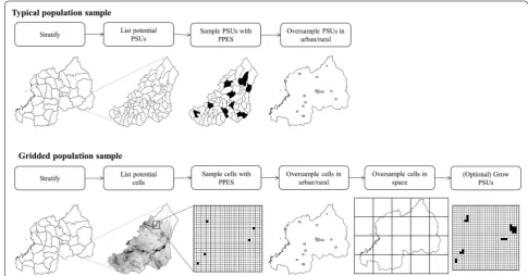
The GridSample package was recently released in R CRAN to generate PSUs for household surveys using gridded population data rather than census data [13]. GridSample supports typical complex sample designs including stratification, oversampling in urban or rural areas, and sampling of different numbers of households within urban and rural areas (Fig. 1). Because grid cells are approximately uniform in size and shape within a country, GridSample also allows for a population sample to be supplemented with a spatial oversample in remote areas which is attractive if survey results will be used to generate small area estimates or make interpolated sur-faces [44] (Fig. 1).

The user needs either two or three datasets to use Grid-Sample. First, a gridded population dataset that covers the study area. Gridded population data are produced in raster file format. A common example of a raster dataset is a photograph which is comprised of pixels, each with a single color value. Similar to a photograph, gridded pop-ulation cells each have one estimated poppop-ulation value. Second, the user provides the boundary of the study area if the sample is not stratified, or boundaries of geographic strata if the sample is stratified. Third, the user option-ally inputs urban/rural area boundaries if urban and rural domains will be represented in the survey. Bounda-ries are commonly formatted as a shapefile, a type of file used to store points, lines, or polygons (areas) and their attributes. GridSample requires that all input datasets are converted to raster format using the same grid cell dimensions as the population dataset. Below, we provide a code example to convert shapefiles to rasters.

The shapefile includes a record for each PSU containing the latitude-longitude coordinate of the PSU centroid (geographic center), and the PSU and strata population counts needed in sample weight calculations.

In the following sections, we provide a technical over-view of the GridSample algorithm workflow; describe how to replicate typical complex survey designs in Grid-Sample; describe the use of population sampling with a spatial oversample; and reproduce an existing DHS sample in GridSample. To support use of GridSample, we provide sample weight calculation instructions, dis-cuss practical limitations, outline areas for future grid-ded population survey research, and offer suggestions to improve the feasibility of fieldwork.

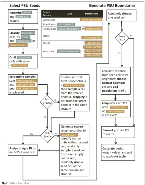
GridSample: technical workflow

GridSample is an R CRAN package with four functions— gs_mode, gs_rasterize, gs_zonal_raster, and gs_sample— though the user only interacts with the main function, gs_sample. GridSample is written for R version 3.2.3 or newer, and requires the following libraries: rgdal (≥1.2– 5), raster (≥2.5–8), data.table (≥1.10.4), rgeos (≥0.3–22), geosphere (≥1.5–5), sp (≥1.2–4), deldir (≥0.1–12), spat-stat (≥1.49–0), and maptools (≥0.8-41). Figure 2 visual-izes how the input datasets and parameters are processed in gs_sample. At a minimum, the user must specify the input gridded population dataset ( population_ras-ter), household sample size (cfg_hh_per_stratum), study area boundary (which is strata_raster, the boundary of a single stratum sample), population size per PSU (cfg_pop_per_psu), and number of households to be sampled per PSU (the urban value cfg_hh_per_ urban is used for all PSUs if a rural value cfg_hh_ per_rural is not specified). Further complexities can be added to the survey design including stratification, oversampling of urban/rural populations, and spatial sampling. GridSample first selects PSU seed cells from the dataset, and then optionally grows each PSU by add-ing neighboradd-ing cells until a minimum geographic size (cfg_max_psu_size) or population size (cfg_pop_ per_psu) is achieved.

Before using gs_sample, the user must rasterize all vector data to match the grid dimensions of the grid-ded population dataset (population_raster). Specifically, the user must rasterize urban/rural bound-aries and strata boundbound-aries. Urban/rural boundbound-aries (urban_raster) may be defined from existing data sources such as Global Urban Footprint (GUF) [45], Global Rural Urban Mapping Project (GRUMP) [36], Global Human Settlement City Model (GHS-SMOD) [46], Modis 500  m urban extents [47], and European Space Agency Land Cover class for urban areas [48]. Alternatively, the user may generate urban/rural extents

by classifying the population density layer ( popu-lation_raster), or by uploading an urban/rural shapefile from another source. Choice of urban/rural boundary is highly dependent on the nature of the sur-vey, as definitions of urban and rural populations dif-fer across countries and disciplines [49]. The strata boundary raster (strata_raster) can be derived from administrative area boundaries, for example Map Library [50] or DIVA-GIS [51], though the user might upload alternative strata boundaries defining, for exam-ple, ecological regions or a program catchment area.

To select PSU seed cells, gs_sample classifies each cell in the gridded population dataset ( popula-tion_raster) by urban or rural location (if cfg_ sample_rururb  =  TRUE and urban_raster is specified), and assigns a stratum ID ( strata_ras-ter). Serpentine sampling is used such that cells are geographically ordered from west-to-east, north-to-south, and sampled based on a random starting cell and a population increment that produces the desired number of PSUs within the stratum, thus facilitating a randomized population-weighted sample. The user may halt the algorithm at this point leaving just one cell per PSU by setting the PSU growth parameter to false (cfg_psu_growth = FALSE).

If the PSU growth parameter is set to true (cfg_psu_ growth = TRUE), gs_sample grows PSUs using a dilation filter routine to enlarge the area around each PSU seed cell by adding neighboring cells one cell at a time until the specified population per PSU parameter is met. From the seed cell, the dilation routine randomly chooses one of the nearest north, east, south, or west cells, and adds that population to the PSU. The routine loops over each PSU adding more population cells each time until each PSU achieves the maximum PSU area in square kilom-eters (cfg_max_psu_size) or total population per PSU value (cfg_pop_per_psu). A valid sample frame has contiguous, non-overlapping potential PSUs. Thus, GridSample restricts PSUs to being contiguous and non-overlapping by drawing voronoi polygons around each seed cell, defining unique areas in which each PSU can grow; the PSU growth routine will not add cells beyond a strata or voronoi polygon boundary.

reproduce an existing sample. The following attributes are needed to calculate sample weights (presented later): number of selected PSUs in stratum (psus_in_stratum), estimated population in stratum (str_pop), and estimated population in PSU (psu_pop).

GridSample: clustered sampling

GridSample supports the first-stage of the typical two-stage cluster design used by DHS, MICS, and LSMS, as well as several other common survey designs. The user defines the desired total population in each PSU (cfg_ pop_per_psu), ranging from 400 to 600 people in typi-cal household surveys. Alternatively, GridSample can be used to select one-stage cluster samples by setting the total population per PSU (cfg_pop_per_psu) equal to the number of households to be sampled per PSU (cfg_hh_per_urban and cfg_hh_per_rural) multiplied by the average household size (available from previous surveys). Likewise, GridSample might be used to select a random sample of households by setting total population per PSU (cfg_pop_per_psu) equal to the average household size, and setting the number of house-holds to be sampled per PSU (cfg_hh_per_urban

and cfg_hh_per_rural) equal to 1. To implement a random sample of households, the user would addition-ally need to use a method to identify a random dwelling within each PSU [8].

GridSample: stratification

Strata should be mutually exclusive geographic areas that cover the entire population. In typical household surveys, sub-national administrative areas such as provinces or dis-tricts serve as strata, and sometimes these areas are further stratified into rural and urban areas. Independent samples will be selected from each stratum allowing strata-level estimates to be compared after the survey. While some gridded population datasets provide estimates of popula-tion by age-group and sex [25, 52, 53] or household pov-erty level [54, 55], GridSample does not currently include a mechanism for non-geographic stratification, though the user could, in principal, sample from gridded population datasets of social-demographic groups.

To generate a geographically stratified sample in GridSample, the user defines strata boundaries with strata_raster, and specifies the sample size per stratum with cfg_hh_per_stratum. This means that if the national sample size is 10,000 households from 5 provinces, then cfg_hh_per_stratum  ==  2000. If the survey were additionally stratified by urban/rural such that there are 10,000 households sampled from 10 strata, then strata_raster should include the boundaries of both urban/rural areas and provinces, and cfg_hh_per_stratum == 1000.

GridSample: urban/rural oversampling

If urban/rural populations are not stratified, they may instead be treated as sub-domains. Sub-domains repre-sent important sub-populations for which reprerepre-sentative statistics are generated from the survey data, and thus each sub-domain should meet the minimum stratum sample size requirement (cfg_hh_per_stratum). If either the urban or rural sub-domain does not include enough households, then the algorithm uses the ordered data frame to choose the next cell from the under-rep-resented sub-domain (from any strata) and swaps out an already selected seed cell of the opposite sub-domain within that stratum. This process repeats until the sample size requirement is met in each sub-domain (cfg_hh_ per_stratum). To implement sub-domain representa-tion in gs_sample, set cfg_sample_rururb == 1 and define urban/rural boundaries (urban_raster).

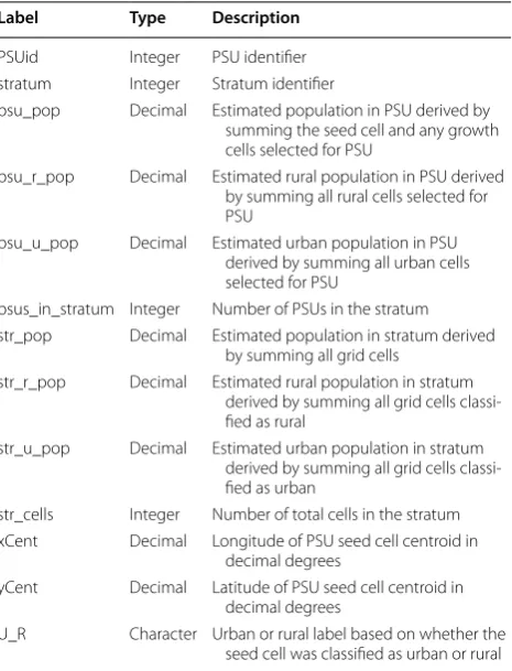
In practice, rural areas may be more difficult and expensive to visit, and thus a greater number of house-holds might be sampled from rural PSUs than urban PSUs. This is why the user may specify different numbers Table 1 Summary of attributes in the output shapefile

Label Type Description

PSUid Integer PSU identifier

stratum Integer Stratum identifier

psu_pop Decimal Estimated population in PSU derived by summing the seed cell and any growth cells selected for PSU

psu_r_pop Decimal Estimated rural population in PSU derived by summing all rural cells selected for PSU

psu_u_pop Decimal Estimated urban population in PSU derived by summing all urban cells selected for PSU

psus_in_stratum Integer Number of PSUs in the stratum str_pop Decimal Estimated population in stratum derived

by summing all grid cells

str_r_pop Decimal Estimated rural population in stratum derived by summing all grid cells classi-fied as rural

str_u_pop Decimal Estimated urban population in stratum derived by summing all grid cells classi-fied as urban

str_cells Integer Number of total cells in the stratum xCent Decimal Longitude of PSU seed cell centroid in

decimal degrees

yCent Decimal Latitude of PSU seed cell centroid in decimal degrees

of households to be sampled from urban PSUs (cfg_hh_ per_urban) and rural PSUs (cfg_hh_per_rural). If the same number of households will be sampled from all PSUs, then the user only needs to specify households to be sampled from urban PSUs (cfg_hh_per_urban).

GridSample: spatial oversampling and other features

Oversampling in space is analogous to oversampling urban/rural sub-domains. To select a sample that is both representative of the population and of space in Grid-Sample, set cfg_sample_spatial == 1 and spec-ify the spatial scale (in square kilometers) at which the sample should be representative ( cfg_sample_spa-tial_scale). For example, cfg_sample_spatial_ scale == 20 means that a coarse grid system with cells 20 km × 20 km will be overlaid on the study area. If a coarse grid cell does not contain a PSU seed cell, then the first cell within the serpentine ordered data frame located inside the course cell will be selected, and another seed cell from the same stratum and sub-domain will be ran-domly dropped. To overcome the issue of slightly smaller grid cells toward the poles, GridSample calculates the area of the centroid (geographic center) grid cell in the study area, and uses that average grid cell size to generate the coarse grid with the correct dimensions.

The spatial scale of the survey is ideally linked to the scale of planned small area estimates. For example, if the sample is stratified by province (level 1 adminis-trate units), and small area estimates will later be gen-erated for districts (level 2 administrative units), then the median size of districts could be used. Determining an appropriate spatial scale may take trial and error. If the country has large areas of sparse population, the user might need to (a) increase the size of the spatial scale (cfg_sample_spatial_scale), or (b) force the algorithm to generate more PSUs in each stratum by increasing the sample size per stratum (cfg_hh_ per_stratum) and/or reduce the number of house-holds sampled in each PSU (cfg_hh_per_urban and cfg_hh_per_rural).

GridSample offers several additional parameters. (1) The user can input a 100 m × 100 m gridded population data-set, and then aggregate cells for the sample frame (e.g. 300  m ×  300  m sample frame cells would be generated by setting cfg_desired_cell_size = 3). Aggregat-ing gridded population estimates usually increases the accuracy of each grid cell. Note that guidance regarding the ideal cell size of gridded population sample frames is not yet available. Other parameters include: (2) minimum population per cell (cfg_min_pop_per_cell) which

will exclude grid cells from the sample frame with less than the specified minimum population, (3) maximum area of the PSU in squared kilometers (cfg_max_psu_ size) to ensure that PSUs can be feasibly enumerated during fieldwork, (4) random number value (cfg_ran-dom_number) to reproduce a previous gridded population sample, and (5) halt the PSU growth process (cfg_psu_ growth = FALSE) discussed in detail below.

Results

We replicated the first-stage sample of the 2010 Rwanda DHS in GridSample. The 2010 Rwanda DHS sampled 12,540 households from 492 PSUs comprising rural villages and urban neighborhoods [56]. The sample was stratified by Rwanda’s 30 districts, urban areas were oversampled by adding 12 PSUs in Kigali’s three districts, and 26 house-holds were sampled from each urban and rural PSU. The average village in Rwanda had 610 occupants according to the sample frame of 14,837 villages/neighborhoods. To rep-licate the 2010 Rwanda DHS in GridSample, we loaded the GridSample package, the raster package to prepare the data for GridSample, and set a working directory:

R> library(gridsample) R> library(raster)

R> library(rgdal) #if uploading own shapefile boundaries R> setwd("C:/User/Project")

Next, we called the Rwanda 2010 UN-adjusted grid-ded population estimates preloagrid-ded in GridSample and also available at the WorldPop website [33]. This data-set was generated from 2002 Rwanda Census block data and 15 spatial covariates using a random forest model with dasymetric redistribution as described in the metadata [57] and cited methods paper [30].

R> population_raster <- raster(paste0(path.package("gridsample"), + "/extdata/RWA_ppp_v2b_2010_UNadj.tif"))

R> plot(population_raster)

R> data(RWAshp)

R> strata_raster <- rasterize(RWAshp,population_raster, + field="ADM2_ID")

R> plot(strata_raster)

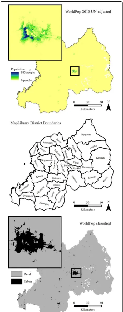
We considered using GUF, Modis or GRUMP to distin-guish urban and rural areas, though we decided that these global models were not well suited for the largely rural context of Rwanda [38]. Instead, we calculated a sensible value to distinguish rural and urban cells directly from the WorldPop population raster. According to the 2012 Cen-sus, the National Institute of Statistics in Rwanda classifies 16% of the population as urban [58]. Thus, we identified the cell density value associated with 16% of the popula-tion living in the most populous cells, and used that value (11 people per 100 m × 100 m cell) to create a binary ras-ter of urban areas (value 1) and rural areas (value 0).

R> total_pop=cellStats(population_raster,stat="sum")

R> urban_pop_value = total_pop*.16 #Table 4, Rwanda 2012 census R> pop_df = data.frame(index = 1:length(population_raster[]),pop = + population_raster[])

R> pop_df = pop_df[!is.na(pop_df$pop),]

R> pop_df = pop_df[order(pop_df$pop,decreasing = T),] R> pop_df$cumulative_pop = cumsum(pop_df$pop) R> pop_df$urban = 0

R> pop_df$urban[which(pop_df$cumulative_pop<=urban_pop_value)] = 1 R> urban_raster <- population_raster >=

+ ceiling(min(subset(pop_df,urban == 1)$pop)) R> plot(urban_raster)

Note that the value used to differentiate urban and rural cells was found with the following code.

R> urb_df=subset(pop_df,urban == 1)

R> ceiling(min(subset(pop_df,urban == 1)$pop))

The gridded population, rasterized strata, and raster-ized urban/rural layers are visualraster-ized in Fig. 3. We used these input data, plus parameters for total household sam-ple size per stratum (cfg_hh_per_stratum = 416), grow PSUs (cfg_psu_growth = TRUE) to a minimum population total per PSU (cfg_pop_per_psu = 610), and household sample size per urban and rural PSU (cfg_ hh_per_urban =  26 and cfg_hh_per_rural = 26), to generate a gridded population sample with the same design as the 2010 DHS. We prevented sampling of cells with very small probability of population (cfg_min_ pop_per_cell  =  0.01), limited the PSU size to 10 km × 10 km (cfg_max_psu_size = 10), and speci-fied the name (sample_name =  ”rwanda_psu_sam-ple”) and file location (output_path = ” C:/User/ Project/data”) to save the output shapefile.

Fig. 3 Input datasets to the Rwanda gridded population sample in

R> psu_polygons=gs_sample(population_raster = population_raster, + strata_raster = strata_raster,

+ urban_raster = urban_raster, + cfg_random_number = , + cfg_desired_cell_size = NA, + cfg_hh_per_stratum = 416, + cfg_hh_per_urban = 26, + cfg_hh_per_rural = 26, + cfg_min_pop_per_cell = 0.01, + cfg_max_psu_size = 10, + cfg_pop_per_psu = 610, + cfg_psu_growth = TRUE, + cfg_sample_rururb = TRUE, + cfg_sample_spatial = FALSE, + cfg_sample_spatial_scale = , + output_path=" C:/User/Project/data", + sample_name="rwanda_psu_sample") R> plot(psu_polygons)

The Rwanda DHS selected 79 urban PSUs and 413 rural PSUs from their census sample frame. Grid-Sample produced a similar sample of 75 urban PSUs and 405 rural PSUs (Table 2) which followed a similar geographic pattern as the Rwanda DHS (Fig. 4) using the WorldPop sample frame. In the GridSample -gen-erated sample [59], the mean population per PSU was 620 people with one outlier that had 1479 people, and the median population was 612 people per PSU. One key difference between the samples was that the DHS added PSUs during the oversample, while GridSample re-distributed PSUs during the oversample, resulting in fewer PSUs. A second key difference was that DHS purposefully oversampled in the Kigali metropolitan area (Gasabo, Kicukiro and Nyarugenge districts) while GridSample oversampled from all urban areas, includ-ing smaller cities in Gisenyi, Cyangugu, and Gikongoro districts.

Discussion

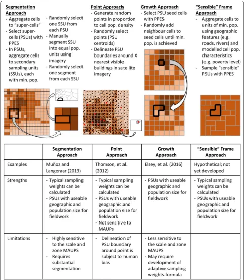
Gridded population sampling methods are in their infancy. Several approaches to first-stage sample selec-tion and to fieldwork have been tried. These approaches are promising but have limitations and require further research. The GridSample R algorithm provides a tool to develop and evaluate emerging gridded population sam-pling methods.

Modifiable Areal Unit Problem

Gridded population sampling is sensitive to the modifia-ble areal unit promodifia-blem (MAUP). A MAUP emerges when an arbitrary spatial unit, such as a grid cell, is used to summarize continuous population characteristics lead-ing to apparently different spatial patterns of that char-acteristic in the population simply by changing the size (scale) or zone (grouping) of the spatial units [60]. In

gridded population sampling, the size and zone of grid cells are likely to influence sampling inclusion probabili-ties, especially when the first-stage sample is based on geographically large grid cells, and/or the population is heterogeneously distributed.

Four general approaches to first-stage sampling with gridded population data are outlined in Fig. 5. First, the segmentation approach involves sampling geographi-cally large PSUs with probability proportionate to esti-mated population size, then segmenting by smaller grid cells [10] or manually delineate smaller areas using sat-ellite imagery [6–10]. GridSample can be used to select large cells by aggregating the input gridded popula-tion dataset. In Myanmar, Muñoz and Langeraar (2013) Table 2 Number of  primary sampling units in  a Demo-graphic and Health Survey and equivalent GridSample sur-vey

District name Alternative name DHS GridSample

Urban Rural Urban Rural

Bugesera Bugesera 16 2 14

Burera Burera 16 1 15

Butamwa Nyarugenge 19 1 15 1

Butare Huye 3 13 3 13

Byumba Gicumbi 2 14 1 15

Cyangugu Rusizi 2 14 5 11

Gakenke Gakenke 16 16

Gasiza Nyabihu 16 1 15

Gatagara Ruhango 3 13 16

Gatsibo Gatsibo 16 16

Gikongoro Nyamagabe 1 15 3 13

Gisagara Gisagara 16 16

Gisenyi Rubavu 1 15 10 6

Gitarama Muhanga 4 12 1 15

Kamonyi Kamonyi 16 16

Kayonza Kayonza 16 16

Kibungo Ngoma 3 13 1 15

Kibuye Karongi 2 14 2 14

Kicukiro Kicukiro 20 13 3

Kigali Gasabo 11 9 8 8

Kirehe Kirehe 16 16

Nogororero Ngororero 16 16

Nyagatare Nyagatare 16 16

Nyamasheke Nyamasheke 16 16

Nyanza Nyanza 4 12 2 14

Nyaruguru Nyaruguru 16 16

Ruhengeri Musanze 2 14 3 13

Rulindo Rulindo 16 1 15

Rutsiro Rutsiro 16 16

Rwamagana Rwamagana 2 14 3 13

aggregated LandScan 1 km × 1 km gridded population estimates to 3 km × 3 km “super” cells for selection of the first-stage sample. Then they grouped 1 km × 1 km grid cells within the selected PSUs to meet a minimum

population threshold, and then randomly sampled one group of cells as a secondary sampling unit (SSU) in each PSU. Finally, they manually segmented SSUs into dozens of areas with roughly equal population based on satellite

imagery, and sampled one segment [10]. As a result, the sample weights were computationally straightforward to calculate because they followed a typical multi-stage sampling approach. Additionally, the final sampling units had sensible boundaries related to features in the real world, making fieldwork feasible. However, sample inclu-sion probabilities of PSUs and SSUs were sensitive to the size and zone of grid cells, which could have smoothed-out or emphasized population density depending on the distribution of the underlying population.

A point approach was used by Thomson and colleagues (2012) using LandScan 1  km ×  1  km gridded popula-tion data in the eastern D. R. Congo. For this survey, the team generated randomly located points within grid cells where the number of points was proportional to esti-mated population. Then they randomly sampled points within strata. Finally, they manually delineated sam-pling units around the nearest dwellings to each point using satellite imagery, ensuring that PSU boundaries were located within cell boundaries [6]. Sample weights were adapted to follow a typical multi-stage sampling approach, the final sampling unit boundaries were sen-sible, making fieldwork feasen-sible, and the use of points prevented any effect of the MAUP. However, the manual delineation of one sampling unit around each point was subject to human bias.

The third approach to gridded population sampling is the growth approach, uniquely available in the Grid-Sample tool. Elsey et  al. [7] in Kathmandu, Nepal used an early version of GridSample to select seed cells from WorldPop’s 100 m × 100 m gridded population dataset, and grew PSUs to a minimum population size. Growing PSUs is likely less sensitive to the zone and scale MAUPs than segmenting large cells because, in the growth approach, the scale of the starting grid cells is closer in geographic and population size to the final sampling unit. However, the correct calculation of sampling inclusion probability weights for the growth approach is unclear. Should sample probability weights be calculated from the grid cell densities, or the densities of final sampling units? Arguments can be made for both approaches. Before dis-cussing two potential sample weight calculations for the growth approach, we describe a hypothetical, but feasi-ble, fourth approach to gridded population sampling.

Perhaps the most ideal gridded population sample frame would group grid cells into “sensible” potential PSUs of similar population size before first-stage sam-pling. Sensible PSU boundaries would be defined in terms of geographic features such as roads, rivers, ridges or valleys that could be easily recognized and navigated in the field. Sensible PSUs would also group similar types of populations, for example, by grid cell mean poverty level. Generation of a sensible gridded population sample

frame has only recently become possible as new tech-niques are developed to estimate population characteris-tics, such as poverty-level or disease status, in a gridded population format [54, 61]. The use of quadtree methods to divide dense population grid squares into four smaller cells can be viewed as a rudimentary first step toward development of sensible potential PSUs [62]. If a grid-ded population sample frame of sensible potential PSUs existed, the survey practitioner would sample units with probability proportionate to estimated size, and calculate typical sampling inclusion probability weights.

The growth approach to gridded population sampling may be conceptualize of as one instance of a sensible frame in which only the boundaries of the sampled PSUs are known, and the boundaries of non-sampled potential PSUs exist but are not drawn. Sample weights calculated from the final PSU population densities are straightfor-ward to calculate, and are provided below.

If, however, the growth approach inclusion probabilities need be calculated from grid cell (rather than final PSU) population densities, then a complex adaptive sample weight needs to be formulated [63]. An adaptive sample weight would account for the estimated population of a given cell, as well as the probability of being grown into a PSU via a neighboring cell. The probability of being grown into a PSU would depend on (a) the estimated populations of neighboring cells, (b) the parameter for PSU maximum geographic size, (c) the parameter for PSU minimum pop-ulation size, and possibly (d) the location of strata bound-aries, and (e) the location of voronoi polygon boundaries between seed cells in a multitude of sample instances. The need for such a complex formulation needs to be evalu-ated, but is beyond the scope of this paper.

Sample weights

probability that PSU i is selected, and then household j is selected—is given by:

where nk is the number of selected PSUs in stratum k, Gk is

the estimated total population in stratum k, gik is the esti-mated population in PSU i in stratum k, mik is the num-ber of households sampled in PSU i and stratum k during fieldwork, and Mik is the number of total households

enu-merated in PSU i and stratum k during fieldwork.

If growth PSUs are manually divided and further sam-pled, weights are calculated in the same way, except that the probability of being in the final sample unit wij.b includes bik, the proportion of households located in the manually-drawn segment, approximated by counting buildings in satellite imagery:

The household response weight—the probability that PSU i is found and sampled, and household j is found and responded—is given by:

where nk number of selected PSUs in stratum k, nk∗ is the

number of found and sampled PSUs in stratum k, mik is the number of selected households in PSU i and stratum k, and mik∗ is the number of found and responded

house-holds in PSU i and stratum k. The individual response weight—the probability that PSU i is found and sampled, then household j is found and responds, and finally that individual q is present and responds—is given by:

where nk is the number of selected PSUs in stratum k, nk∗

is the number of found and sampled PSUs in stratum k,

mik is the number of selected households in PSU i and stratum k, mik∗ is the number of found and responded

households in PSU i and stratum k, and uijk is the number of eligible individuals in household j in PSU i and stra-tum k, and uijk∗ is the number of responded individuals

in household j in PSU i and stratum k. The household sample weight wij is comprised of the household selection weight and household response weight:

Assuming that all eligible individuals (e.g., all women age 15–49) will be interviewed in the selected

(1)

wij._b=

1

Pi×Pj(i) =

Gk/gik

n_k ×

Mik

m_ik

(2)

wij._b= Gk/gik

n_k ×

Mik

m_ik ×

1

b_ik

(3)

wij._r= 1

Pi._r×P_j._r(i) = nk

nk∗×

mik

mik∗

(4)

wijq._{r =}

1

Pi._r×P_j._r(i)×P_q._r(ji)

= nk

n_k∗×

mik m_ik∗×

uijk u_ijk∗

(5)

wij =wij._b×wij._r

households, the individual sample weight wijq is com-prised of the household selection weight and individual response weight:

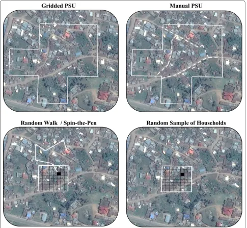
Fieldwork

Four approaches are available for survey fieldwork with GridSample output. These four approaches are visualized in Fig. 6, and described below.

Gridded PSUs

This option uses gridded PSU boundaries which have squared corners and no relation to geographic or administrative features in the real world. This approach was used in a two-stage cluster survey of households in Kathmandu, Nepal [7]. The team used OpenStreet-Map™, a crowd sourced online map of roads, building locations, and other features, via an Android application on mobile phones to digitally map households within PSUs. OpenStreetMap™ enumeration was chosen over typical pen-and-paper mapping, in part, because half of their PSUs were already mapped in OpenStreetMap™. Households (defined as a group of people who share a cook pot) were fully enumerated by knocking on doors and talking to neighbors ensuring that lower-income households who shared an apartment were not under-sampled. The team encountered, sometimes substantial, differences in the number of households per PSU than were expected from the WorldPop sample frame, so they planned to interview every 10th _household regard-less of PSU size to achieve a probability sample. The team cited geographic accuracy in field maps, feasibil-ity of mapping in dense, complex urban environments, leveraging of existing data, and the ability to contrib-ute to a crowd-sourced resource as reasons to use this approach [7].

We support the use of OpenStreetMap™ enumera-tion, especially for urban settings where OpenStreet-Map™ data are likely to exist. However, we strongly recommend that implementers employ a method to anonymize buildings added to the crowd-sourced map such that interviewed PSUs cannot be identified. In areas where buildings have already been mapped in OpenStreetMap™, minor edits will not reveal PSU loca-tions. However, in areas of the map without building and road locations, implementers should consider mapping beyond the edges of the PSU boundaries so that gridded PSU shapes do not suggest a gridded household survey. Furthermore, if OpenStreetMap™ data are sparse in the survey region, implementers should consider enumerat-ing a number of fake PSUs to preserve the anonymity of interviewed communities. Specific guidelines for Open-StreetMap™ enumeration are not yet available.

(6)

Manually‑drawn PSUs

A second approach to implement gridded population samples is to manually draw PSUs around random points within seed cells, or to manually segment gridded sam-pling units using detailed satellite imagery. Manually-drawn PSUs were used in a one-stage cluster survey in eastern D. R. Congo [6] and a two-stage cluster sur-vey in Myanmar [10]. A key benefit of this approach is that PSUs follow sensible boundaries such as rivers and roads, which are easily identified in both satellite images and in the field. Because manually-drawn PSUs are easily identifiable, field teams are flexible to use hand-sketched

pen and paper maps, printed maps of satellite imagery or OpenStreetMap™ features, or digital maps for field navi-gation and household enumeration.

Non‑probability samples

Random-walk and “spin-the-pen” sampling methods result in non-probability samples of the population and are thus not recommended by surveyors [64–66]. None-theless, these and similar methods are often used in rapid or high-security field assessments because they are cheaper and faster to implement than typical two-stage cluster samples. Random-walk and spin-the-pen gridded

sampling methods were used in rapid assessments in Iraq [8] and Myanmar [11]. In both studies, gridded popula-tion datasets were considered to be more accurate sam-ple frames than other available population data. Because random-walk and spin-the-pen methods do not lead to probability samples, we do not provide sample probabil-ity weights.

Simple random sample of households

Researchers sometimes perform simple random samples of households in small study areas—for example, a refu-gee camp or a single city—by digitizing dwelling point locations in a satellite image and sampling points at ran-dom [67–71]. While a simple random sample of house-holds has not been conducted using gridded population sampling, it would be straightforward to implement. Grid cells would be sampled with probability proportionate to estimated size, and the growth algorithm could optionally be switched off to generate single cell PSUs. Then a single dwelling would be randomly chosen within selected cells, either from mapping all dwellings or using a method like the one described by Galway and colleagues in Iraq [8]. In the Iraq study, the team overlaid a 10 m × 10 m mini-grid on Google Earth™ satellite imagery within the seed cell, and then randomly selected one mini-grid unit. If the 10  m mini-grid unit covered a building, the build-ing was selected for samplbuild-ing, otherwise the process was repeated until the first building was randomly identified in the imagery. If the randomly selected building had multiple households or was non-residential, one nearby household could be randomly selected as describe by Siri and colleagues in Kenya [66]. A simple random sample of households would not require sample weights.

Limitations

Gridded population data are increasingly used as an alternative survey sample frame in countries where cen-sus data are outdated or inaccurate. Gridded population sample frames may also be used in lieu of census data for surveys that need to be representative of both population and of space, and where PSUs of a specific population size are needed. Next we discuss six areas where research is underway, or needed, to address limitations of gridded population sampling.

Accuracy of gridded population sample frame

The first major concern in gridded population sampling is the accuracy of the underlying gridded population data. Gridded population sampling has been tried by a number of survey implementers in circumstances of outdated or inaccurate census data, however the accu-racy of gridded population datasets are varied, and often unquantified. Accuracy of publically available top-down

gridded population data is dependent on several model components: (1) accuracy of the input census data, (2) the geographic scale of the input census data (e.g. cen-sus tract-level vercen-sus district-level), (3) the age, accu-racy, and type of model covariate data, and (4) the model algorithm itself. The geographic scale of the output grid also matters for measurement of accuracy; grid cell estimates in a 1 km × 1 km gridded population dataset will almost always be more accurate than grid cells in a 100 m × 100 m gridded population dataset. Model errors are difficult to estimate, and to even conceptualize, for gridded population datasets that rely on simple disaggre-gation approaches, as they are essentially gridded repre-sentations of the input census data [24]. While prediction errors can be calculated for gridded population datasets derived from complex modelling techniques, WorldPop is the only dataset to include errors [see, for example, 56]. However, it is unclear how survey implementers can use prediction errors to quantify or improve the accuracy of household survey sample frames.

Numerous studies have evaluated the accuracy of grid-ded population estimates against ground-collected set-tlement locations [72], against census data available at a finer-scale than the census data used in the model [29,

73–76], and by comparing old and new gridded popu-lation datasets where the new dataset uses updated or finer-scale population data [38]. Still this evidence is not sufficient to assess the accuracy of a specific top-down gridded population dataset. Given the number of compo-nents that contribute to gridded population model error, future research should utilize simulation studies to test the effects of various model components on gridded pop-ulation estimates. These studies should also reframe how the estimate errors are addressed (e.g. rather than ask “how much error is there around the estimate for each cell of size X?”, researchers should ask “how many cells need to be aggregated to achieve an error of Y?”).

Modifiable areal unit problem

Second, segmentation and growth approaches to sample unit selection might be subject to bias from the MAUP. Simulation studies should be used to quantify the effects of grid cell sizes and groupings on PSU selection probabilities. Additionally, development of geographically and socially sensible sample frames with gridded population data should be pursued. The ability to create a sensible gridded population sample frame is highly dependent on availability of fine scale, accurate environmental data and gridded esti-mates of population social-health characteristics.

Adaptive PSU sample weights

adaptive sample weights should be used, and if so, how to formulate them. These questions can be evaluated with statistical theory and simulation studies.

Availability of satellite imagery

Fourth, all of the approaches to gridded population sam-pling described here are dependent on access to fine-res-olution satellite imagery with good visibility of dwellings without extensive tree-cover or cloud-cover. Existing gridded population samples have been implemented in cities, camps, deserts, savannah, and deforested farm-lands; methods for implementing gridded population samples have not been described for forested areas.

Concealing PSU locations in publications and crowd‑sourced maps

Fifth, gridded population samples that use crowd-sourced maps in fieldwork must guarantee anonymity of survey respondents and their communities. Crowd-sourced maps can be incredibly valuable for field navigation and house-hold enumeration, though the technology and protocols to support survey activities are limited. Standard proto-cols have not yet been established to conceal survey PSU locations when mapping buildings and roads in a crowd-sourced platform such as OpenStreetMap™. Furthermore, we are not aware of any applications that allow survey enu-merators to both update OpenStreetMap™ and separately store a confidential household listing linked to building locations, which interviewers would need to identify sam-pled households. As in any survey, PSU boundaries and centroid point locations should not be shared publically to protect the anonymity of respondents and their com-munities. PSU point locations can be published if they are randomly geo-displaced following methods like those used by MeasureDHS [77]. The MeasureDHS project publishes PSU centroid coordinates that are displaced up to 2  km in urban areas, and up to 5 km in rural areas, with one in every 100th rural point displaced up to 10 km.

Fieldwork feasibility

The sixth concern of gridded population sampling is feasibility of fieldwork. While there are multiple rea-sons to use gridded population sampling, protocols to use these methods in the field need further develop-ment. What is the enumeration protocol in a PSU that falls on two sides of a river where there is not a nearby bridge to cross? Should buildings be enumerated if they are intersected by the PSU boundary? Given that grid-ded PSU boundaries do not follow sensible geographic or administrative boundaries, recent satellite imagery is almost certainly needed during enumeration. What is the minimum image resolution required for sampling in rural versus urban areas? How recent should the satellite

imagery be? What are the tradeoffs of using digital enu-meration methods over paper-based methods? While the use of smart phones or tablets to digitally enumerate PSUs increases the cost and skill requirements among enumerators, it may also reduce the time and increase the accuracy of enumeration compared to pen-and-paper methods. Multiple issues related to cost, time, accuracy, technology, and staff skill requirements to implement gridded population surveys need to be evaluated.

Conclusions

The GridSample R package facilitates further research into the promising field of gridded population sampling. Gridded population sampling is an attractive alterna-tive to typical sampling methods when census data are outdated or inaccurate. GridSample supports standard complex survey designs including clustered sampling, stratification, and oversampling in urban or rural areas. GridSample additionally allows users to oversample in space, and to specify a desired population size of sampling units. We show that GridSample can be used to replicate a DHS in Rwanda, providing evidence of a similar number of primary sampling units with similar population sizes in urban and rural areas. We also summarize four ways in which gridded population samples have been imple-mented in the field, and provide sample weight calcula-tions for GridSample output. Finally, we discuss several areas of current and future research into gridded popula-tion sampling which can benefit from this tool.

Abbreviations

CRAN: Comprehensive R Archive Network; DHS: Demographic and Health Sur-vey; EA: Enumeration area; GHSL: Global Human Settlement Layer; GPW: Grid-ded Population of the World; GRUMP: Global Rural–Urban Mapping Project; GUF: Global Urban Footprint; LSMS: Living Standards Measurement Survey; MAUP: modifiable areal unit problem; MICS: Multiple Indicator Cluster Survey; PPES: probability proportionate to estimated size; PSU: primary sampling unit; SDG: sustainable development goals; SSU: secondary sampling unit; UNEP: United Nations Environment Programme.

Authors’ contributions

DRT drafted the user requirements, conceptualized the first part of the GridSample algorithm related to PSU selection, tested the software, and wrote the first draft of the manuscript. FRS conceptualized the second part of the GridSample algorithm related to PSU growth and wrote the first draft of the R code. NWR refined the code and added to it conceptually, for example, by introducing voronoi polygons to ensure contiguous, non-overlapping PSUs. AJT facilitated team introductions, provided key technical guidance during the algorithm development, and contributed extensive revisions to the manu-script. MCC provided key practitioner guidance during the algorithm develop-ment, and contributed extensive revisions to the manuscript. All authors read and approved the final manuscript.

Additional file

Author details

1 _{Department of Social Statistics and Demography, University of} South-ampton, Building 58, Southampton SO17 1BJ, UK. 2 _{WorldPop, Department} of Geography and Environment, University of Southampton, Building 44, Southampton SO17 1BJ, UK. 3 _{Flowminder Foundation, Roslagsgatan 17,} 11355 Stockholm, Sweden. 4 _{Department of Geography and Geosciences,} Uni-versity of Louisville, 200 E Shipp Ave, Louisville, KY 40208, USA. 5 _Department of Global Health and Population, Harvard T.H. Chan School of Public Health, 665 Huntington Ave, Boston, MA 02115, USA.

Acknowledgements

Special thanks to Tomas Bird, Nikos Tzavidis, Shoaib Ali, Alesandro Sorichetta, Dale Rhoda, and Kristen Himelein who all provided helpful insights about sample weight calculations and spatial sampling. We also thank the two anonymous reviewers who asked questions and gave input that improved this manuscript.

Competing interests

The authors declare that they have no competing interests.

Availability of data and materials

The input data used in this analysis is available with the GridSample R package: Thomson DR, Ruktanonchai NW, Stevens FR, Castro M, Tatem AJ. 2017. grid-sample: Tools for Grid-Based Survey Sampling Design. R package version 0.1.2. https://CRAN.R-project.org/package=gridsample. The output dataset from the GridSample R package is available online: Thomson DR. 2017. GridSample output: 2010 Rwanda DHS. Harvard Dataverse. http://dx.doi.org/10.7910/DVN/MSCJOD.

Funding

This work is supported by funding from the Bill & Melinda Gates Founda-tion (OPP1106427). DRT is supported by funding from the UK Economic and Social Research Council (Grant Number ES/J500161/1). FRS is supported by funding from the Bill and Melinda Gates Foundation (OPP1134076) with initial development supported by the National Science Foundation (0801544). NWR is supported by funding from Clinton Health Access Initiative. AJT is supported by funding from NIH/NIAID (U19AI089674), the Bill and Melinda Gates Foundation (OPP1106427, 1032350, OPP1134076, OPP1094793), the Clinton Health Access Initiative (which supports NR), National Institutes of Health, and a Wellcome Trust Sustaining Health Grant (106866/Z/15/Z). MCC thanks the support from the Department of Global Health and Population. The funders had no role in study design, data collection and analysis, decision to publish, and preparation of the manuscript.

Publisher’s Note

Springer Nature remains neutral with regard to jurisdictional claims in pub-lished maps and institutional affiliations.

Received: 27 March 2017 Accepted: 4 July 2017

References

1. Global Health Data Exchange (GHDx). Institute for Health Metrics and Evalu-ation, Seattle. 2017. http://ghdx.healthdata.org/. Accessed 10 Mar 2017. 2. Global Health Observatory data repository. World Health Organization,

Geneva. 2017. http://apps.who.int/gho/data/node.home. Accessed 10 Mar 2017.

3. Food Security Analysis: Assessments. World Food Programme, Rome. 2017. http://vam.wfp.org/?_ga=1.230081818.764469399.1485248139. Accessed 3 Mar 2017.

4. HDX Database v.1.8.3. Humanitarian data exchange. 2017 https://data. humdata.org/. Accessed 10 Mar 2017.

5. Consumer Panels. Neilsen. 2017 http://www.nielsen.com/id/en/solu-tions/measurement/consumer-panels.html. Accessed 10 Mar 2017. 6. Thomson DR, Hadley MB, Greenough PG, Castro MC. Modelling

strategic interventions in a population with a total fertility rate of 8.3: a cross-sectional study of Idjwi Island, DRC. BMC Public Health. 2012. doi:10.1186/1471-2458-12-959.

7. Elsey H, Thomson DR, Lin RY, Maharjan U, Agarwal S, Newell J. Addressing inequities in urban health: do decision-makers have the data they need? Report from the urban health data special session at international confer-ence on urban health, Dhaka 2015. J Urban Health. 2016. doi:10.1007/ s11524-016-0046-9.

8. Galway L, Bell N, Sae AS, Hagopian A, Burnham G, Flaxman A, et al. A two-stage cluster sampling method using gridded population data, a GIS, and Google EarthTM imagery in a population-based mortality survey in Iraq. Int J Health Geogr. 2012. doi:10.1186/1476-072X-11-12.

9. Hagopian A, Flaxman AD, Takaro TK, Esa Al Shatari SA, Rajaratnam J, Becker S, et al. Mortality in Iraq associated with the 2003–2011 war and occupation: findings from a national cluster sample survey by the Uni-versity Collaborative Iraq Mortality Study. PLoS Med. 2013. doi:10.1371/ journal.pmed.1001533.

10. Muñoz J, Langeraar W. A census-independent sampling strategy for a household survey in Myanmar. 2013. http://winegis.com/images/census- independent-GIS-based-sampling-strategy-for-household-surveys-plan-of-actionremoved.pdf. Accessed 10 Mar 2017.

11. Sollom R, Richards AK, Parmar P, Mullany LC, Lian SB, Iacopino V, et al. Health and human rights in Chin State, Western Burma: a population-based assessment using multistaged household cluster sampling. PLoS Med. 2011. doi:10.1371/journal.pmed.1001007.

12. ICF International. Demographic and Health Survey sampling and house-hold listing manual. 2012. https://dhsprogram.com/pubs/pdf/DHSM4/ DHS6_Sampling_Manual_Sept2012_DHSM4.pdf. Accessed 10 Mar 2017. 13. Thomson DR, Ruktanonchai NW, Stevens FR, Castro M, Tatem AJ.

Grid-Sample: tools for grid-based survey sampling design. R package version 0.1.2. 2017. https://cran.r-project.org/package=gridsample. Accessed 10 Mar 2017.

14. United Nations Children’s Fund (UNICEF). Designing and selecting the sample. In: Multiple indicator cluster surveys round 4. 2012. http://mics. unicef.org/tools?round=mics4. Accessed 10 Mar 2017.

15. United Nations (UN). Designing household survey samples: practical guidelines. Studies in methods series F No. 98. 2005. https://unstats. un.org/unsd/demographic/sources/surveys/Handbook23June05.pdf. Accessed 10 Mar 2017.

16. ICF International. Demographic and Health Survey sampling and household listing manual. 2012. https://dhsprogram.com/pubs/pdf/ DHSM4/DHS6_Sampling_Manual_Sept2012_DHSM4.pdf. Accessed 10 Mar 2017.

17. Grosh ME, Munoz J. A manual for planning and implementing the Living Standards Measurement Study Survey. LSMS Working Paper No. 126. 1996. http://documents.worldbank.org/curated/ en/363321467990016291/pdf/multi-page.pdf. Accessed 10 Mar 2017. 18. ICF International. Survey organization manual for Demographic and Health Surveys. 2012. http://dhsprogram.com/pubs/pdf/DHSM10/ DHS6_Survey_Org_Manual_7Dec2012_DHSM10.pdf. Accessed 13 May 2017.

19. Shannon HS, Hutson R, Kolbe A, Stringer B, Haines T. Choosing a survey sample when data on the population are limited: a method using Global Positioning Systems and aerial and satellite photographs. Emerg Themes Epidemiol. 2012. doi:10.1186/1742-7622-9-5.

20. Kamanga A, Renn S, Pollard D, Bridges DJ, Chirwa B, Pinchoff J, et al. Open-source satellite enumeration to map households: planning and targeting indoor residual spraying for malaria. Malar J. 2015. doi:10.1186/ s12936-015-0831-z.

21. Lohr SL. Sampling: design and analysis. 2nd ed. Boston: Brooks/Cole; 2009.

22. Census dates for all countries. 2020 World Population and Housing Cen-sus Programme, United Nations Statistics Division, Geneva. 2016. https:// unstats.un.org/unsd/demographic/sources/census/censusdates.htm. Accessed 10 Mar 2017.

23. Carr-Hill R. Missing millions and measuring development progress. World Dev. 2013. doi:10.1016/j.worlddev.2012.12.017.

24. GADM. Known problems. In: Global administrative areas v.2.8. 2015. http://www.gadm.org/problems. Accessed 3 Mar 2017.

26. Environmental Data Explorer: Gridded Population of the World. United Nations Environment Programme, Nairobi. 2006. http://geodata.grid. unep.ch/. Accessed 10 Mar 2017.

27. Balk D, Brickman M, Anderson B, Pozzi F, Yetman Y. Mapping global urban and rural population distributions: estimates of future global population distribution to 2015. 2005. http://www.fao.org/docrep/009/a0310e/ a0310e00.htm. Accessed 10 Mar 2017.

28. Pesaresi M, Ehrlich D, Florczyk AJ, Freire S, Julea A, Kemper T, et al. Operat-ing procedure for the production of the Global Human Settlement Layer from Landsat data of the epochs 1975, 1990, 2000, and 2014. 2016. http:// publications.jrc.ec.europa.eu/repository/handle/JRC97705. Accessed 10 Mar 2017.

29. Facebook Connectivity Lab and Center for International Earth Science Information Network—CIESEN—Columbia University. High Resolution Settlement Layer (HRSL) [Internet]. Source imagery for HRSL 2016 Digi-talGlobe. 2016. https://ciesin.columbia.edu/data/hrsl/. Accessed 10 Mar 2017.

30. Stevens FR, Gaughan AE, Linard C, Tatem AJ. Disaggregating census data for population mapping using random forests with remotely-sensed and ancillary data. PLoS ONE. 2015. doi:10.1371/journal.pone.0107042. 31. Dobson JE, Bright EA, Coleman PR, Durfee RC, Worley BA. LandScan: a

global population database for estimating populations at risk. Photo-gramm Eng Remote Sens. 2000;66(7):849–57.

32. Azar D, Engstrom R, Graesser J, Comenetz J. Generation of fine-scale population layers using multi-resolution satellite imagery and geospatial data. Remote Sens Environ. 2013. doi:10.1016/j.rse.2012.11.022. 33. WorldPop Data. WorldPop, University of Southampton, Southampton UK.

2017. http://www.worldpop.org.uk/data/data_sources. Accessed 10 Mar 2017. 34. Gridded Population of the World v4. Center for International Earth

Science Information Network, Columbia University, New York. 2016. http://sedac.ciesin.columbia.edu/data/collection/gpw-v4/sets/browse. Accessed 10 Mar 2017.

35. GHS Population Grid. European Commission, Brussels. 2017. http://ghsl. jrc.ec.europa.eu/ghs_pop.php. Accessed 18 May 2017.

36. Gridded Rural Urban Mapping Project v1. Center for International Earth Science Information Network, Columbia University, New York. 2006. http://sedac.ciesin.columbia.edu/data/set/grump-v1-population-count/ data-download. Accessed 10 Mar 2017.

37. LandScan Data Availability. Oak Ridge National Laboratories, Oak Ridge, Tennessee. 2017. http://www.ornl.gov/sci/landscan/landscan_data_avail. shtml. Accessed 02 Feb 2017.

38. Tatem AJ, Noor AM, Hay SI. Assessing the accuracy of satellite derived global and national urban maps in Kenya. Remote Sens Environ. 2005. doi:10.1016/j.rse.2005.02.001.

39. Linard C, Alegana V, Noor AM, Snow RW, Tatem AJ. A high resolution spa-tial population database of Somalia for disease risk mapping. Int J Health Geogr. 2010. doi:10.1186/1476-072X-9-45.

40. Tatem AJ. Mapping the denominator: spatial demography in the meas-urement of progress. Int Health. 2014. doi:10.1093/inthealth/ihu057. 41. Lu X, Wrathall DJ, Sundsøy PR, Nadiruzzaman M, Wetter E, Iqbal A, et al.

Detecting climate adaptation with mobile network data in Bangladesh: anomalies in communication, mobility and consumption patterns during cyclone Mahasen. Clim Change. 2016. doi:10.1007/s10584-016-1753-7. 42. Wilson R, Zu Erbach-Schoenberg E, Albert M, Power D, Tudge S,

Gonzalez M, et al. Rapid and near real time assessments of popula-tion displacement using mobile phone data following disasters: the 2015 Nepal earthquake. PLoS Curr. 2015. doi:10.1371/currents.dis. d073fbece328e4c39087bc086d694b5c.

43. Deville P, Linard C, Martin S, Gilbert M, Stevens FR, Gaughan AE, et al. Dynamic population mapping using mobile phone data. Proc Natl Acad Sci. 2014. doi:10.1073/pnas.1408439111.

44. Gething P, Tatem A, Bird T, Burgert-Brucker CR. Creating spatial interpola-tion surfaces with DHS data. DHS Spatial Analysis Reports 11. 2015. http:// dhsprogram.com/pubs/pdf/SAR11/SAR11.pdf. Accessed 10 Mar 2017. 45. Global Urban Footprint. DLR Earth Observation Center, Weßling. 2017.

http://www.dlr.de/eoc/en/desktopdefault.aspx/tabid-11725/20508_read-47944/. Accessed 10 Mar 2017.

46. Global Human Settlement City Model (GHS-SMOD). European Commission, Brussels. 2017. http://ghsl.jrc.ec.europa.eu/faq.php. Accessed 10 Mar 2017.

47. Schneider A, Friedl MA, Potere D. Mapping global urban areas using MODIS 500-m data: new methods and datasets based on “urban ecore-gions”. Remote Sens Environ. 2010. doi:10.1016/j.rse.2010.03.003. 48. Climate Change Institute Download Data. European Space Agency, Paris.

2016. http://maps.elie.ucl.ac.be/CCI/viewer/. Accessed 10 Mar 2017. 49. McIntyre NE, Knowles-Yánez K, Hope D. Urban ecology as an

interdiscipli-nary field: differences in the use of “urban’’ between the social and natural sciences. In: Marzluff JM, Shulenberger E, Endlicher W, Alberti M, Bradley G, Ryan C, et al., editors. Urban ecology: an international perspective on the interaction between humans and nature. Boston: Springer; 2008. 50. Map Library. Map Maker Ltd, Campbeltown. 2007.

http://www.mapli-brary.org/library/stacks/Africa/index.htm. Accessed 10 Mar 2017. 51. DIVA-GIS. Hijmans R, Davis. 2016. http://www.diva-gis.org/gdata.

Accessed 10 Mar 2017.

52. Tatem AJ, Campbell J, Guerra-Arias M, de Bernis L, Moran A, Matthews Z. Mapping for maternal and newborn health: the distributions of women of childbearing age, pregnancies and births. Int J Health Geogr. 2014. doi:10.1186/1476-072X-13-2.

53. Alegana VA, Atkinson PM, Pezzulo C, Sorichetta A, Weiss D, Bird T, et al. Fine resolution mapping of population age-structures for health and development applications. J R Soc Interface. 2015. doi:10.1098/ rsif.2015.0073.

54. Steele JE, Sundsøy RP, Pezzulo C, Alegana VA, Bird TJ, Blumenstock J, et al. Mapping poverty using mobile phone and satellite data. R Soc Interface. 2017. doi:10.1098/rsif.2016.0690.

55. Ruktanonchai CW, Ruktanonchai NW, Nove A, Lopes S, Pezzulo C, Bosco C, et al. Equality in maternal and newborn health: modelling geographic disparities in utilisation of care in five East African countries. PLoS ONE. 2016. doi:10.1371/journal.pone.0162006.

56. National Institute of Statistics of Rwanda (NISR), Ministry of Health (MOH), ICF International. Rwanda Demographic and Health Survey 2010. 2012. http://www.measuredhs.com/pubs/pdf/FR259/FR259.pdf. Accessed 10 Mar 2017.

57. WorldPop. Rwanda population map metadata report. 2013. http://www. worldpop.org.uk/data/WorldPop_data/AllContinents/RWA-POP_meta-data.html. Accessed 10 Mar 2017.

58. National Institute of Statistics of Rwanda (NISR). Fourth population and housing census. Thematic Report: population size, structure and distribu-tion. 2012. http://statistics.gov.rw/old/publications/rphc4-thematic-report-population-size-structure-and-distribution. Accessed 10 Mar 2017. 59. Thomson DR. GridSample output: 2010 Rwanda DHS. Harvard Dataverse.

2017. doi:10.7910/DVN/MSCJOD.

60. Openshaw S. The modifiable areal unit problem. Norwick: Geo Books; 1983.

61. Bosco C, Alegana V, Bird T, Pezzulo C, Bengtsson L, Sorichetta A, Steele J, Hornby G, Ruktanonchai C, Ruktanonchai N, Wetter E, Tatem AJ. Exploring the high-resolution mapping of gender-disaggregated development indicators. J R Soc Interface. 2017. doi:10.1098/rsif.2016.0825. 62. Lagonigro R, Oller R, Martori JC. A quadtree approach based on

Euro-pean geographic grids: reconciling data privacy and accuracy. SORT. 2017;41(1):139–58.

63. Thompson SK. Adaptive cluster sampling. J Am Stat Assoc. 1990;85(412):1050–9.

64. Working Group for Mortality Estimation in Emergencies. Wanted: studies on mortality estimation methods for humanitarian emergen-cies, suggestions for future research. Emerg Themes Epidemiol. 2007. doi:10.1186/1742-7622-4-9.

65. Cutts FT, Claquin P, Danovaro-Holliday MC, Rhoda DA. Monitoring vacci-nation coverage: defining the role of surveys. Vaccine. 2016. doi:10.1016/j. vaccine.2016.06.053.

66. Luman ET, Worku A, Berhane Y, Martin R, Cairns L. Comparison of two survey methodologies to assess vaccination coverage. Int J Epidemiol. 2007. doi:10.1093/ije/dym025.

67. Siri JG, Lindblade KA, Rosen DH, Onyango B, Vulule JM, Slutsker L, et al. A census-weighted, spatially-stratified household sampling strategy for urban malaria epidemiology. Malar J. 2008. doi:10.1186/1475-2875-7-39. 68. Wampler PJ, Rediske RR, Molla AR. Using ArcMap, Google Earth, and