Vol. 9, No. 2, 2017 Article ID IJIM-00691, 9 pages Research Article
Convergence of Numerical Method For the Solution of Nonlinear
Delay Volterra Integral Equations
M. Zarebnia ∗†, L. Shiri‡
Received Date: 2015-04-28 Revised Date: 2015-10-14 Accepted Date: 2016-10-16 ————————————————————————————————–
Abstract
In this paper, Solvability nonlinear Volterra integral equations with general vanishing delays is stated. So far sinc methods for approximating the solutions of Volterra integral equations have received considerable attention mainly due to their high accuracy. These approximations converge rapidly to the exact solutions as number sinc points increases. Here the numerical solution of nonlinear delay Volterra integral equations is considered by two methods. The methods are developed by means of the sinc approximation with the single exponential (SE) and double exponential (DE) transformations. These numerical methods combine a sinc collocation method with the Newton iterative process that involves solving a nonlinear system of equations. The existence and uniqueness of numerical solutions for these equations are provided. Also an error analysis for the methods is given. So far approximate solutions with polynomial convergence have been reported for this equation. These methods improve conventional results and achieve exponential convergence. Numerical results are included to confirm the efficiency and accuracy of the methods.
Keywords: Nonlinear Volterra integral equations; General delays; Sinc-collocation; Convergence anal-ysis.
—————————————————————————————————–
1
Introduction
D
ein scientific fields such as physics, biology,lay Volterra integral equations arise widely ecology, control theory, etc. Due to the prac-tical application of these equations, they must be solved successfully with efficient numerical ap-proaches. In recent years, there have been exten-sive studies in convergence properties and stabil-ity analyses of numerical methods for them, see, for example, [12,14]. The numerical solutions of∗Corresponding author. [email protected], Tel: 09113819121.
†Department of Mathematics, University of Mohaghegh Ardabili, Ardabil, Iran.
‡Department of Mathematics, University of Mohaghegh Ardabili, Ardabil, Iran.
integral equations with delays have also been dis-cussed by several authors such as Brunner [2] and Linz Wang [7].
Sinc methods for approximating the solutions of Volterra integral equations have received consid-erable attention mainly due to their high ac-curacy. These approximations converge rapidly to the exact solutions as number sinc points in-creases. Systematic introduction of these meth-ods can be found in [11]. In [13] sinc-collocation method is emplyed to solve Hammerstein Volterra integral equations, but it does not provide exis-tence and uniqueness of the sinc-collocation solu-tion. In this paper we extend the analytical and numerical techniques used in [13] to nonlinear in-tegral equations with general vanishing delay and also show that the sinc-collocation solution exist
and it is unique. In addition to we give an error analysis.
The main objective of the current study is to im-plement the sinc-collocation method for nonlinear Volterra integral equation of the form
y(t) =g(t) +
∫ θ(t)
0
K(t, s, y(s))ds,
t∈I := [0, T], (1.1)
the delay function θ is subject to the following conditions:
(D1) θ(0) = 0, andθis strictly increasing on the interval I;
(D2) θ(t)≤t,t∈I;
(D3) θ∈Cd(I) for some d≥0.
We will refer to a θ that satisfies (D1) as a vanishing delay function (or, in short, a
vanishing delay). The linear case, θ(t) = qt =
t−(1−q)t =: t−τ(t) (0 < q < 1) (propor-tional delay) is also known as the pantograph de-lay function [6]. In this paper we consider van-ishing delay but our methods can be use with nonvanishing delay too.
Several methods have been already presented to the numerical solution of (1.1) for the special case pantograph i.e. θ(t) =qt, for example you can see [2, 3]. We propose two numerical algorithms in order to solve the delay integral equation (1.1) whereθ(t) is more general than pantograph. Our motivation comes from the fact that equa-tion (1.1) may be viewed as a generalizaequa-tion of the equation encountered in the mathematical mod-eling of electric pantograph dynamics and a par-titioning problem in number theory [8]
y(t) =g(t) +
∫ qt
0
k(t, s)y(s)ds.
The layout of this paper is as follows. In Sec-tion 2, the solvability of the Eq. (1.1) is stated. Section3outlines some of the main properties of sinc function that is necessary for the formulation of the delay integral equation. Sinc-collocation method is considered in Section 4. In section 5, we analyze the existence and uniqueness of nu-merical solutions. In Section 6, the orders of scheme convergence using the new approache are described. Finally, Section7contains the numer-ical experiments.
2
Existence and uniqueness of
solutions
In the present section, we state the solvability of nonlinear integral equations with vanishing delay. To state the following theorem we will adopt the notation
D:={(t, s) : 0⩽s⩽t⩽T},
ΩB :={(t, s, y) : (t, s)∈D, y∈R
and |y−g(t)|⩽B},
and we set MB := max{|K(t, s, y)|: (t, s, y) ∈
ΩB}.
Theorem 2.1 Assume:
(a) g∈C(I) andK ∈C(ΩB);
(b) θ(t)is subject to the assumptions (D1)-(D3);
(c) K satisfied the Lipschitz condition
|K(t, s, y)−K(t, s, z)|⩽LB|y−z|,
for all (t, s, y),(t, s, z)∈ΩB.
Then:
(i) The Picard iteration yn(t) exist for alln⩾1.
They are continuous on the interval I0 :=
[0, δ0], where
δ0:= min{T, B/MB},
and they converge uniformly on I0 to a
so-lution y ∈ C(I0) of the nonlinear Volterra
integral equation (1.1).
(ii) This solution y is the unique continuous so-lution on I0.
Proof. The above result is also related to an exis-tence and uniqueness result in [3]. His proof tech-niques are readily extended to the general delay function in whichθ(t) is subject to the conditions (D1)-(D3). We omit the details. □
3
Review of the sinc
approxima-tion
These are discussed thoroughly in [11]. The sinc basis functions are given by
S(j, h)(z) = sinc(z−jh
h ),
j= 0,±1,±2, . . . (3.2)
where
sinc(z) =
{ sin(πz)
πz , z̸= 0;
1, z= 0,
andh is a step size appropriately chosen depend-ing on a given positive integer N, and j is an integer and (3.2) is called the jth sinc function. Originally, sinc approximation for a functionu is expressed as
u(t)≈
N ∑
j=−N
u(jh)S(j, h)(t), t∈R. (3.3)
The above approximation is valid on R, whereas the Eq. (1.1) is defined on finite interval [0, T]. The Eq. (3.3) can be adapted to approximate on general intervals with the aid of appropriate variable transformations t=ϕ(x). As the trans-formation functionϕ(x) appropriate single expo-nential (SE) and double expoexpo-nential (DE) trans-formations are applied. The single exponential transformation and its inverse can be introduced respectively as below
ψSE(x) =
T ex
1 +ex,
ϕSE(t) = ln(
t T−t).
In order to define a convenient function space, the strip domain Dd ={z∈ C :|Imz|< d} for some
d > 0 is introduced. When incorporated with the SE transformation, the conditions should be considered on the translated domain
ψSE(Dd) ={z∈ C:|arg(
z
T −z)|< d}.
The following definitions and theorems are con-sidered for further details of the procedure.
Definition 3.1 Let D be a simply connected do-main which satisfies(a, b)⊂Dandα andc1 be a
positive constant. ThenLα(D)denotes the family
of all functions u∈Hol(D) which satisfy
|u(z)|⩽c1|Q(z)|α (3.4)
for all z in D where Q(z) = (z−a)(b−z).
The next theorem shows the exponential conver-gence of the SE-sinc approximation.
Theorem 3.1 Let u ∈ Lα(D), let N be a
posi-tive integer, and let h be selected by the formula
h =
√ πd
αN, then there exists positive constant c2,
independent of N, such that
sup
t∈(a,b)
|u(t)−
N ∑
j=−N
u(ψSE(jh))S(j, h)(ϕSE(t))|
⩽c2 √
N e− √
πdαN.
The error analysis of the SE-sinc indefinite inte-gration has been given in [9].
Theorem 3.2 Let uQ ∈ Lα(D) for d with 0 <
d < π. Let h =
√ πd
αN. Then there exists a
con-stant c3, which is independent of N, such that
sup
t∈(a,b) |
∫ t
a
u(s)ds−h
N ∑
j=−N
u(ψSE(jh))ψ′SE(jh)
J(j, h)(ϕSE(t))|⩽c3e−
√
πdαN (3.5)
where
J(j, h)(x) = 1 2 +
∫ x
h−j
0
sin(πt)
πt dt.
The double exponential transformation can be used instead of the single exponential transfor-mation. DE-transformation and its inverse are
ψDE(x) =
b−a
2 tanh(
π
2sinh(x))
+b+a 2 ,
ϕDE(t) = ln[
1
πln( t−a b−t)
+
√
1 +
{
1
π ln
(
t−a b−t
)}2
].
This transformation maps Dd onto the domain
ψDE(Dd) ={z∈ C :|arg[
1
πln( t−a b−t)
+
√
1 +{1
πln( t−a b−t)}
2]|< d}.
The following theorem describes the extreme accuracy of DE-sinc approximation when u ∈
Theorem 3.3 Let u ∈ Lα(ψDE(Dd)) for d with
0 < d < π2, N be a positive integer and h is se-lected by the formula h = ln(2dN/αN ). Then there exists a constant c4 which is independent of N,
such that
sup
t∈(a,b)
|u(t)−
N ∑
j=−N
u(ψDE(jh))
S(j, h)(ϕDE(t))|⩽c4e−πdN/ln(2dN/α).
If we use the DE transformation instead of the SE transformation, the DE-sinc quadrature is achieved. The rate of convergence is accelerated as the next theorem states.
Theorem 3.4 ([9]) Let uQ ∈ Lα(ψDE(Dd)) for
d with0 < d < π2. Let α′ =α−ϵ for 0< ϵ < α, N be a positive integer with N > α′/(2d), and h is selected by the formula
h= ln(2dN/α
′)
N .
Then there exists a constant c5 which is
indepen-dent of N, such that
sup
t∈(a,b) |
∫ t
a
u(s)ds−h
N ∑
j=−N
u(ψDE(jh))ψDE′ (jh)
J(j, h)(ϕDE(t))|⩽c5e−πdN/ln(2dN/α
′)
.
4
Sinc-collocation method
In the present section, we apply sinc-collocation method to solve Eq. (1.1) which we state again for the convenience of the reader:
y(t) =g(t) +
∫ θ(t)
0
K(t, s, y(s))ds,
t∈I := [0, T],
ift= 0 we have y(0) =g(0). For ease of calcula-tion, we employ the transformation
u(t) =y(t)−T −t
T g(0),
in this case u(0) = 0. Then the above problem becomes
u(t) =f(t) +
∫ θ(t)
0
K1(t, s, u(s))ds (4.6)
where
f(t) :=g(t)−T −t
T g(0),
K1(t, s, u(s)) :=K(t, s, u(s) +
T−t T g(0)).
Now, letu(t) be the exact solution of (4.6).
4.1 SE-sinc scheme
The approximate solutionUNSE is considered that has the form
USE
N (t) =
N ∑
j=−N
u(ψSE(jh))S(j, h)(ϕSE(t))
+u(T)wSE(t), t∈[0, T] (4.7)
we choose wSE(t) so that above formula
interpo-late function u at the points
tSEj =
{
ψSE(jh), j=−N, . . . , N;
T, j=N + 1,
then
wSE(t) =
1
T(t−
N ∑
j=−N
tSEj S(j, h)(ϕSE(t))).
We replace approximate solution (4.7) in (4.6). Substituting t=tSEk ,k=−N, . . . , N+ 1
uSEk =f(tSEk ) +
∫ θ(tSE
k )
0
K1(tSEk , s,
N ∑
j=−N
uSEj S(j, h)(ϕSE(s))
+uSEN+1wSE(s))ds, (4.8)
we approximate the integral in above equation by the quadrature formula presented in (3.5)
∫ θ(tSE
k )
0
K1(tSEk , s, N ∑
j=−N
uSEj
S(j, h)(ϕSE(s)) +uSEN+1wSE(s))ds
=h
N ∑
l=−N
ψSE′ (lh)J(l, h)(ϕSEk )
K1(tSEk , tSEl , uSEl ),
where
ϕSEk :=ϕSE(θ(tSEk )).
Thus Eq. (4.8) is written as
uSEk =f(tSEk ) +h
N ∑
l=−N
ψ′SE(lh)
J(l, h)(ϕSEk )K1(tSEk , tSEl , uSEl ), (4.9)
This linear system of equations is equivalent to (4.6). By solving this system, the unknown coefficients uSEk are determined. We rewrite the nonlinear system (4.9) in matrix form
ASE(uSE) =uSE, (4.10)
where
[ASE(uSE)]k,l:=f(tSEk ) +hψ′SE(lh)J(l, h)(ϕSEk )
K1(tSEk , tSEl , uSEl ), k, l=−N, . . . , N+ 1,
uSE:= [uSE−N, . . . , uSEN+1]t.
4.2 DE-sinc scheme
The DE-sinc case is focused on in this part. Sim-ilar to the SE-sinc method, the approximate so-lutionUNDE can be defined as follow
UDE
N (t) =
N ∑
j=−N
uDEj S(j, h)(ϕDE(t))
+uSEN+1wDE(t), t∈[0, T]. (4.11)
By applying (4.11) and setting its collocation on 2N + 2 sampling points at t = tDEk , for k =
N, . . . , N+1,in Eq. (4.6), the following nonlinear system
ADE(uDE) =uDE, (4.12)
is achieved. By solving this system, the unknown coefficients in uDE have been found.
5
Existence and uniqueness of
the sinc-collocation solution
In this section, we study the existence and uniqueness of the solution to (4.10) and (4.12). It is necessary to bound the basis function J(j, h). The next lemma gives the bound.
Lemma 5.1 ([11]) For x ∈ R, the function J(j, h)(x) is bounded by
|J(j, h)(x)|⩽1.1.
Theorem 5.1 Assume that K1, and f in the
nonlinear Volterra equation (4.6) are continuous and
|K1(t, s, u(t))−K1(t, s, v(t))|
< L|u(t)−v(t)|.
Then the nonlinear algebraic systems (4.10) and (4.12) have a unique solution.
Proof. Using Lemma 5.1 and continuty K1 we
have
∥ASE(u)−FSE∥
∞
= max
k |h
N ∑
l=−N
ψSE′ (lh)J(l, h)(ϕSEk )
K1(tSEk , tSEl , uSEl )|
⩽1.1hsup
x |
ψ′(x)|
N ∑
l=−N
|K1(tSEk , tSEl , uSEl )|
⩽1.1he−N h
N ∑
l=−N
|K1(tSEk , tSEl , uSEl )|
⩽1.1he−N h(2N + 1)M,
where M is upper bound of |K1(t, s, u(t))| and
FSE := [f(tSE−N), . . . , f(tSEN+1)]t.
By using fixed point theorem, this proves that the nonlinear system has a solution in the closed ball with centerFSEand radius 1.1hT(2N+1)M. It may be shown that, if K1 is Lipschitz with
re-spect to u(t), the solution is unique. For suppose that u,v are two possible solutions
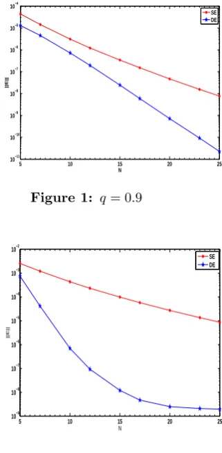
5 10 15 20 25
10−11 10−10 10−9
10−8
10−7 10−6 10−5
10−4
N
||E||
SE DE
Figure 1: q= 0.9
5 10 15 20 25
10−9 10−8 10−7 10−6 10−5 10−4 10−3 10−2
N
||E||
SE DE
∥u−v∥∞=∥ASE(u)− ASE(v)∥∞ = max k h N ∑
l=−N
ψSE′ (lh)J(l, h)(ϕSEk )
K˙1(t˙kˆSE,t˙lˆSE,u˙l)-K˙1(t˙kˆSE,t˙lˆSE,v˙l)
⩽1.1he−N hmax
k N ∑
l=−N
|K1(tSEk , tSEl , ul)
−K1(tSEk , tSEl , vl)|
⩽1.1he−N hmax
k N ∑
l=−N
L|ul−vl|
⩽1.1he−N h(2N+ 1)L∥u−v∥∞
<∥u−v∥∞,
because limN→∞he−N h(2N + 1) = 0, we can
write the last inequality for some N. It follows that∥u−v∥∞ vanishes and there is thus unique-ness.
The similar conclusions are achieved for DE case. □
6
Convergence analysis
The convergence of the two sinc-collocation meth-ods which are introduced in the previous sections is discussed in the present section. We first con-sider the SE case. It is assumed that uSE is the exact solution of Eq. (4.10) and uSE
(m) is an
ap-proximation ofuSEobtained from Newton’s iter-ative process.
In the following theorem, we will find an upper bound for the error.
Theorem 6.1 LetUNSE(t)is the approximate so-lution of integral equation (4.6). Then there ex-ists a constant c5 independent of N such that
sup
t∈(0,T)
|u(t)− UNSE(t)|
⩽c5 √
N e− √
πdαN. (6.13)
Proof. The error between u and USE
N can be
expressed by
u(t)− UNSE(t)
=f(t) +
∫ θ(t)
0
K1(t, s, u(s))
− N ∑
j=−N
uSEj S(j, h)(ϕSE(t))
−uSEN+1wSE(t)
=f(t) +
∫ θ(t)
0
K1(t, s, u(s))
− N ∑
j=−N
{
f(tSEj ) +h
N ∑
l=−N
ψSE′ (lh)
J(l, h)(ϕSEj )K1(tSEj , tSEl , uSEl ) }
S(j, h)(ϕSE(t))− {
f(tSEN+1)
+h
N ∑
l=−N
ψSE′ (lh)J(l, h)(ϕSEN+1)
K1(tSEN+1, tSEl , uSEl ) }
wSE(t)
=f(t)−
N ∑
j=−N
f(tSEj )S(j, h)(ϕSE(t))
−f(tSEN+1)wSE(t) +
∫ θ(t)
0
K1(t, s, u(s))
−h
N ∑
j=−N
N ∑
l=−N
ψ′SE(lh)J(l, h)(ϕSEj )
K1(tSEj , tSEl , ulSE)S(j, h)(ϕSE(t))
−h
N ∑
l=−N
ψSE′ (lh)J(l, h)(ϕSEN+1)
K1(tSEN+1, tlSE, uSEl )wSE(t)
=c1 √
N e− √
πdαN +c
2 √
N e− √
πdαN
+c3h √
N e− √
πdαN
=c5 √
N e−√πdαN.
Because wSE(tSEj ) = 0 for j =−N, . . . , N, when
we use Theorem 3.1we obtain
N ∑
l=−N
ψSE′ (lh)J(l, h)(ϕSEN+1)
K1(tSEN+1, tlSE, uSEl )wSE(t)
=c3 √
N e− √
πdαN.
If we replace the SE transformation ϕSE by DE
in Theorem , then the similar conclusions are achieved for DE case.
Theorem 6.2 LetUNDE(t)is the approximate so-lution of integral equation (4.6). Then there ex-ists a constant c6 independent of N such that
sup
t∈(0,T)
|u(t)− UNDE(t)|⩽c6e−πdN/ln(2dN/α).
In the following we are trying to discuss the conditions under which Newtons method is con-vergent. For this reason we will state and prove the following theorem.
Theorem 6.3 Assume uSE is the exact solution of the nonlinear system (4.9), and hypotheses of Theorem5.1are satisfied. Also, suppose that ∂K1
∂u
is Lipschitz with respect to u. Then there exist δ > 0 and h > 0 such that if ∥uSE(0) −uSE∥⩽ δ,
the Newton’s sequence {uSE(m)} for any h ∈ (0, h)
is well-defined and convergence to uSE. Further-more, for some constant l with lδ < 1, we have the error bounds
∥uSE(m)−uSE∥⩽ (lδ)
2m
l .
Proof. We must solve the nonlinear system
u− A(u) = 0.
The Newton method reads as follow. Choose an initial guessu0; form= 0,1, . . ., compute
u(m+1) =u(m)−[I − A′(u(m))]−1
[u(m)− A(u(m))], (6.14)
we know that
[A′(u)]k,l =hψ′(lh)J(l, h)(ϕSEk )
∂K1
∂u (t
SE
k , tSEl , uSEk ),
k, l=−N . . . , N,
[A′(u)]N+1,l = 0, l=−N . . . , N,
using Lemma 5.1 and differentiable K1, there
exists a c > 0 so that |[A′(u)]k,l|< ch and then ∥A′(u)∥< 1 whenever h is sufficiently small. In
other words, there is a h > 0 so that for any
h < h matrix (I − A′(u)) has a uniformaly bounded inverse.
The conclusion is straightforwardly achievable by applying Theorem 5.4.1 in [1] and the above discussion. □
In the following theorem, we summarize the conclusions of theorems proved in this section.
Theorem 6.4 Assume that uis an isolated solu-tion of Eq. (4.6), Furthermore, UNSE and uSEN,(m) are the solutions of Eqs. (4.9) and (6.14), re-spectively. Suppose that hypotheses of Theorems6
and 6.3are satisfied. Then there exists a positive constant C(m) independent of N and dependant on m such that
∥u−uSEN,(m)∥⩽C(m)√NlnN e−
√
πdαN.
Proof. The conclusion is obtained by using the triangular inequality and conclusions of Theorems 6and 6.3. □
The proof of the similar theorem goes almost in the same way as in the SE case.
Theorem 6.5 Assume that uis an isolated solu-tion of Eq. (4.6), Furthermore, UNDE and uDEN,(m) are the solutions of Eqs. (4.12) and (6.14), re-spectively. Suppose that hypotheses of Theorems
6.2and6.3are satisfied. Then there exists a pos-itive constant C(m) independent of N and depen-dant on m such that
∥u−uDEN,(m)∥⩽C(m)e−πdN/ln(2dN/α).
7
Illustrative examples
In this section, the theoretical results of the previ-ous sections are used for two numerical examples. The numerical experiments are implemented in
Matlab. In these examples, Newton’s method is iterated until the accuracy 10−8 is obtained. It is assumed thatα= 1. Thedvalues are π2 and
π
4 for the SE-sinc and DE-sinc methods,
respec-tively. The errors of the two methods for N = 5, 10, 15, 20 and 25 are reported. These tables show that increasing N the error significantly is reduced. As expected, the tables show that the convergence rate of the DE-sinc method is faster than the SE-sinc scheme.
Example 7.1 We consider the following panto-graph Volterra integral equation
y(t) =g(t) +
∫ qt
0
(x+t)[u(t)]3dt,
g(t) chosen so that its exact solution is y(t) =
Table 1: Values of∥E∥∞ for Example7.1
N 5 10 15 20 25
SE 4.4085E-5 3.1099E-6 3.4367E-7 4.7006E-8 7.7329E-9 DE 1.3091E5 7.2505E-7 2.4544E-8 7.1655E-10 2.2621E-11
Table 2: Values of∥E∥∞ for Example7.2
N 5 10 15 20 25
SE 2.5315E-3 4.3114E-4 9.8027E-5 2.7038E-5 8.6518E-6 DE 7.4395E-4 6.9632E-7 1.2007E-8 2.4890E-9 1.9521E-9
5 10 15 20 25
10−11
10−10
10−9
10−8
10−7
10−6
10−5
10−4
N
||E||
SE DE
Figure 3: Example7.1,q= 0.9
Example 7.2 Consider the following equation
y(t) =g(t) +
∫ tr
0
2ste−y(s)2ds,
with g(t) =te−t2r has the solution y(t) =t. The errors of the method for r = 0.01 are reported. Table 2 shows the numerical results.
8
Conclusion
We propose two numerical methods based on the sinc function, the SE-sinc and DE-sinc, in order to solve the nonlinear delay integral equation (Eq. (1.1)) where θ is general function. Our methods have been shown theoretically and numerically that it is extremely accurate and achieve expo-nential convergence with respect to N. These two methods have some strengths and weaknesses. In comparison with each other, as the theorems show, it is understood that the SE-sinc formu-las are applicable to larger cformu-lasses of functions than the DE-sinc formulas, whereas the DE-sinc formulas are more efficient for well-behaved func-tions.
References
[1] K. E. Atkinson, W. Han, Theoretical Nu-merical Analysis: A Functional Analysis Framework,Springer, New York, (2001).
[2] H. Brunner, Iterated collocation methods for Volterra integral equations with delay arguments, Math. Comput. 62 (1994) 581-599.
[3] H. Brunner, Collocation Methods for Volterra Integral and Related Functional Equations, Cambridge, (2004).
[4] A. M. Denisov, A. Lorenzi, Existence results and regularisation techniques for severely ill-posed integrofunctional equa-tions, Boll. Un. Mat. Ital. 11 (1997) 713-731.
[5] S. Haber, Two formulas for numerical in-definite integration, Mathematics of Com-putation 60 (1993) 279-296.
[6] A. Iserles, On the generalized pantograph functional differential equation, European J. Appl. Math. 4 (1993) 1-38.
[7] P. Linz, R. L. C. Wang, Error bounds for the solution of Volterra and delay equa-tions, Appl. Numer. Math. 9 (1992) 201-207.
[8] W. Liu, J. C. Clements, On Solutions of Evolution Equations with Proportional Time Delay, Int. J. Differ. Equ. Appl. 4 (2002) 229-254.
and Sinc indefinite integration, Mathemati-cal Engineering TechniMathemati-cal Reports 2009-01, The University of Tokyo, (2009).
[10] F. Stenger, Handbook of Sinc Numerical Methods, Springer, New York, (2011).
[11] F. Stenger, Numerical Methods Based on Sinc and Analytic Functions,Springer, New York, (1993).
[12] K. Yang, R. Zhang, Analysis of contin-uous collocation solutions for a kind of Volterra functional integral equations with proportional delay, Comput. Appl. Math.
236 (2011) 743-752.
[13] M. Zarebnia, J. Rashidinia, Convergence of the Sinc method applied to Volterra inte-gral equations, Appl. Math. 5 (2010) 198-216.
[14] K. Zhang, J. Li, H. Song, Collocation meth-ods for nonlinear convolution Volterra inte-gral equations with multiple proportional delays, Appl. Math. Comput. 218 (2012) 10848-10860.
Mohammad Zarebnia is an As-sociate Professor in Numerical Analysis at the University of Mo-haghegh Ardabili, Ardabil, Iran. He received PHD degree in Ap-plied Mathematics (Numerical Analysis) from the Iran Univer-sity of Science and Technology. His research in-terests include Numerical Analysis, Numerical so-lution of ODEs, PDEs, IEs and Image Processing.