Vol. 11, No. 1, 2019 Article ID IJIM-0910, 8 pages Research Article
A Method for Calculating the Marginal Rate in the FDH Model
M. Mirzaei ∗, S. Kordrostami †‡, AR. Amirteimoori §, M. G. Chegini ¶
Received Date: 2016-07-15 Revised Date: 2017-10-16 Accepted Date: 2016-11-01
————————————————————————————————–
Abstract
The concept of trade-off reviews the rate of marginal substitution of inputs and outputs onto the efficient frontier; moreover, marginal rates of substitution (MRS) are important quantities for analysts and managers. In the current study, by changing Asmilds (2004) method, an algorithm has been found that can be used to calculate the marginal rate of the free disposal hull (FDH) model. An empirical study on 20 Iranian bank branches has been presented to illustrate the proposed approach.
Keywords: Data envelopment analysis (DEA); Free disposal hull (FDH); Marginal rate.
—————————————————————————————————–
1
Introduction
T
oedge of trade-offs among activities in thatManage an organization, having a knowl-organization is necessary; as an instance, to in-crease the production rate of a specific output in an organization, officials at the organization should calculate the amount of additional neces-sary input and estimate how much of an input (or output) should increase when the corresponding input (or output) decreases. Another important point not to forget is that in mathematical eco-nomics, it is very convenient for in mathematical economics, it is very convenient formathemati-∗Department of Mathematics, Lahijan Branch, Islamic
Azad University, Lahijan, Iran.
†Corresponding author. [email protected],
Tel:+98(911)1346054.
‡Department of Mathematics, Lahijan Branch, Islamic
Azad University, Lahijan, Iran.
§Department of Applied Mathematics, Rasht Branch,
Islamic Azad University, Rasht, Iran.
¶Department of Management, Rasht Branch, Islamic
Azad University, Rasht, Iran.
cians to operate in terms of efficient surfaces, support hyperplanes, pareto-efficient facets, ref-erence sets, and production correspondences [4]. As a short definition, data envelopment analy-sis (DEA) provides a mathematical programming method for estimating the best practice frontiers and evaluating the relative efficiency of different entities. In fact, DEA is a tool for assessing past performances as part of the management control function and has been widely used to measure and analyze the relative efficiencies of various types of decision making units, such as banks and univer-sity departments, which possess shared functional goals with incommensurate inputs and outputs [10].
One research issue that has attracted consider-able attention in DEA is the problem of determin-ing the marginal rates of the substitution (MRS) of inputs and outputs. With this end in view, the current study discusses how to calculate MRS for efficient decision making units (DMUs) in an ex-treme point in FDH models. Looking at literature of DEA gives us fascinating results; for example, Huang, et al. [6] proposed a general method for
calculating the rates of the change of the outputs to the inputs along the efficient surface of the DEA production set. Rosen et al. [12] studied the problem of MRS on efficient frontier and pre-sented a general framework for the calculation of the trade-offs between two variables in DEA. Cooper et al. [4] proposed an algorithm to search through the extreme points for cost improvements in the case of given prices or relative weights and constant outputs and thus considered non-marginal trade-offs as well.
Asmild et al. [3] applied the envelopment form of the BCC (Banker, Charnes and Cooper) model to calculate the marginal rates of substitution. They also developed some methods for evaluating larger trade-offs or non-marginal rates of substi-tution between variables in DEA. Khoshandam et al. [9] proposed a production function in which a group of variables were changed in a given direc-tion, and then they calculated the effect of this change on some throughput.
Mirzaei et al. [11] showed that the binding effi-cient supporting surfaces of an effieffi-cient point may be used to define the alternative marginal rates of substitutions. Having these studies in mind, the aim of the current paper is to present a tech-nique that enables DEA practitioners to deter-mine rates of substitution and transformation in FDH models. This research discusses how to cal-culate the MRS for efficient DMUs in an extreme point in FDH models. With this end in view, the researchers generalize the work of Asmild et al. [3] to conduct the analysis of MRS in FDH mod-els.
The rest of the paper is structured as follows: Next section provides the original FDH model and its linearization. Section 2 introduces our proposed method to obtain marginal rates of sub-stitution in the FDH model and the trade-off analyses which are illustrated by a simple DEA problem. In Section 3, the marginal rate of sub-stitution of one input and one output for 20 Ira-nian bank branches (DMUs) will be conducted with the use of the proposed method of the cur-rent paper. Conclusions will be presented in Sec-tion 4.
2
Free Disposal Hull (FDH)
Model and Linearization
2.1 The FDH model
The figure of the production possibility set plays an important role in determining the model that we want to use. We know the frontier of the pro-duction possibility set approximates the produc-tion funcproduc-tion. We also know that the producproduc-tion function shows relationship between the tive resources used by an organizations produc-tion (input) and the products or services obtained (output) at the same timeregardless of the price. By accepting the postulates, including observa-tion, convexity, monotonicity and minimum ex-trapolation [c.f. Banker and Thrall (1992)], pro-duction possibility set with constant returns to scale can be defined as follows:
Tc={(x, y) :x≥
∑n
j=1λjxj, y ≤
∑n
j=1λjyj,
λj ≥0, j = 1,2, ..., n}
(2.1) But in some issues, the convex combination of decision making units does not make sense, be-cause the reference units in the CCR (Charnes, Cooper and Rhodes) and BCC models are the convex combination of several decision making units. The main motivation for the appearance of the FDH step model is to make sure that the efficiency will be achieved only on the basis of real observations. So, each of the units must be either involved in the construction of the virtual unitλj (share of unit j)or one or not involved in
that construction,λj is zeroin other words,λj = 0
or 1.
The explanation of the discussion above is sim-ilar to the computation of the efficiency of differ-ent aircraft engines. In the CCR and BCC mod-els, a set of assessment is compared to the vir-tual unit. For example, the expression 12A+12B
on engine efficiency and many real life issues is meaningless. So, the difference between the FDH model and classical models is that technology does not limit itself to the convexity principle. This stance of these models looks attractive, be-cause it can be more in tune with the realities of everyday life.
for the construction of production possibility set, the convex combination of two production pos-sibilities does not necessarily belong to the pro-duction possibility set. So accepting the postu-lates, including observation, monotonicity, possi-bility and minimum extrapolation, the produc-tion possibility set of theF DHc model is defined
as follows:
P P SF DHc = ∪n
j=1{(x, y) :x≥λijxj,
y≤λijyj, λij ≥0} (2.2)
The output-oriented FDH model can be com-pactly written as follows:
M axθ
s.t.
n
∑
j=1
λjxj ≤xk
n
∑
j=1
λjyj ≥θyk
n
∑
j=1
λj = 1
λj ∈ {0,1}, j= 1,2, ..., n (2.3)
where, λis the intensity Boolean vector, andθ
is the free variable and is continuous.
The efficient surface is a staircase based on those given DMUs that are not dominated by other given DMUs. Thus, the efficiency analysis is done relative to the other given DMUs instead of a hypothetical efficiency frontier. This has an advantage that the achievement goal for an inef-ficient DMU given by its efinef-ficient reference point will be more credible than in the cases of CCR and the BCC models. The reference point will simply be one of the already existing operating DMUs.
2.2 Linearization
We know that the above model is a mixed integer programming one, and it is difficult to use. Al-though there is no need to solve a linear program-ming problem for solving the FDH model, only a paired comparison is the optimal solution. But it has its own drawbacks including the assumption of strictly positive input and output vectorsa very difficult assumption in practical issues. Moreover,
among these models none comes to the slack vari-ables, and this is a non-linear model. In order to avoid these problems, the linear reformulation of the output-oriented FDH model (2.3) is used as given in [1] as follows:
M ax
n
∑
j=1
θj
s.t. θjyro−yrjλj+s+rj = 0,∀r,∀j,
(xij −xio)λj+s−ij = 0,∀i,∀j, n
∑
j=1
λj = 1,
λj ≥0, s+rj ≥0, s−ij ≥0 (2.4)
A DM U0 is FDH efficient if θ0∗ = 1. It is clear
that the FDH model is a special case of DEA models. With the FDH formulation, each DMU is evaluated by comparing it to the other DMUs on a one-to-one basis [5].
3
Marginal Rates Substitution
in the FDH Model
Consider a general process, where a vector of out-puts Y = (y1, y2, ..., ys)∈ Rs+ is produced by a
vector of inputs X = (x1, x2, ..., xm)∈ Rm+. To
simplify the developments, let us write the inputs and outputs as a single vector of throughputs
Z = (z1, ..., zn) = (−X, Y)T =
(
−x1, ...,−xn
y1, ..., yn
)
. We assume that the production frontier, given by the graph{Z|F(z) = 0}is monotonic, contin-uous, piecewise, differentiable, and concave. Note that frontiers constructed with DEA satisfy these conditions in general; in fact, the production fron-tier in DEA may be represented as follows:
T ={Z|Zλ≥z, 1Tλ= 1} (3.5)
whereλis n-dimensional intensity vector and1 is n-dimensional unity vector.
The marginal substitution rate of throughputjto throughputkat a point on the frontierz0is defined
as partial derivative as
M RSjk(z0) =
∂z0j
∂z0k
|z0 =−
∂F/∂z0k
∂F/∂z0j
|z0, j̸=k
This partial derivative gives the increase in throughput j when throughputk is increased by one unit and all the other throughputs are kept constant. When the throughputs correspond to two inputs, the rate (3.6) is usually referred to as the technical rate of substitution (marginal rate of technical substitution); when they corre-spond to two outputs, it is called the marginal rate of transformation; and when zj andzk refer
to an output and an input, it is often called the marginal productivity (marginal impact), which is in accordance with what is said in microeco-nomics.
The marginal rates of substitution of through-put j to throughput k, at the point z0 on the
FDH frontier can be calculated with the use of the following procedure:
1- Determine a small increment h for the kth throughput.
2- Obtain the optimum value of ∑nj=1z∗0jby solving the linear programming problem below, which is resulted from increasing (or decreasing) thekth throughput to h.
Opt
n
∑
j=1
z0∗j
s.t. Zλ≥z0∗
1Tλ= 1
z∗0l=z0l, l̸=j, k
z∗0k=z0k+h
λ≥0 (3.7)
In fact, applying one of the following linear pro-gramming problems for the FDH model in terms of what trade-offs to be done with input and out-put gives us:
M ax
n
∑
i=1
yi∗0
s.t.(xio+h−xij)λj ≥0,∀i,∀j,
yrjλj ≥yi∗0,∀r,∀j,
n
∑
j=1
λj = 1,
λj ≥0,∀j.
M in
n
∑
i=1
x∗i0
s.t.(yrj−yi0−h)λj ≥0,∀r,∀j
,
−xijλj ≥ −x∗i0,∀i,∀j, n
∑
j=1
λj = 1,
λj ≥0,∀j.
These linear programming problems are solved for the jth component of the throughput vector when thekth component is increased (decreased) by the small quantityh, such that it still remains on the FDH frontier.
3- Compute the finite marginal rate of substi-tution from the right:
M RSjk+(z0) =
∑n
j=1z∗0j−z0j
h
If h is replaced by −h′ and steps two and three are repeated, the marginal rate of substitution will be obtained from the left. Note that we do not have |h′ |=h, because the FDH model is a special case of interval data model, and it is not necessary for the increments of left and right to be equal.
3.1 Illustration of Marginal Changes
This approach for calculating the marginal rates of substitution is illustrated by a simple numeri-cal example with four DMUs; each unit has one input and one output:
Fig. 1:
Suppose that X = (6,8,14,10) and Y = (2,4,5,3) and consider k = 2 for an output-oriented FDH model; then we will have:
M ax θ+ε(s++s−)
s.t.2λ1+ 4λ2+ 5λ3+ 3λ4−s+ = 4θ,
6λ1+ 8λ2+ 14λ3+ 10λ4+s−= 8,
The linearization equivalent ([1]) will, in this case, be like what follows:
M ax
4
∑
h=1
θh+ε 4
∑
h=1
(s+h +s−h)
s.t.2λ1−s+1 −4θ1 = 0,
4λ2−s+2 −4θ2 = 0,
5λ3−s+3 −4θ3 = 0,
3λ4−s+4 −4θ4 = 0,
(6−8)λ1+s−1 = 0,
(8−8)λ2+s−2 = 0,
(14−8)λ3+s−3 = 0,
(10−8)λ4+s−4 = 0, 4
∑
h=1
λh = 1,
λ, s+h, s−h ≥0, θhf ree.
We have to solve this problem; (λ∗1, λ∗2, λ∗3, λ∗4) = (0,1,0,0) and(θ1∗, θ∗2, θ3∗, θ∗4)
= (0,1,0,0). That means that the second unit is efficient. Similarly, it can be shown that the 1th and 3th units are as efficient and inefficient as the 4th unit.
Now suppose that Z0= (yi∗0,0)T and
Z = [Yh,−(Xh−xk)]T = [Yh,−(Xh−8)]T
=
(
2
−(6−8)
4
−(8−8)
5
−(14−8)
3
−(10−8)
)
In fact, (−x0, y0)T = (−8,4)T, and consider
the rate of substitution M RS(y)(−x), that is, the
change inyresults from a marginal change in−x. 1. Let h= 2.
2. The value of ∑4i=1y∗i0 resulted from increasing−x0 by h to −6 (i.e. Z0∗ =
(∑4i=1y∗i0,−6)T) is found by
M ax
4
∑
i=1
yi∗0
s.t.
2λ1 ≥y10∗
4λ2 ≥y20∗
5λ3 ≥y30∗
3λ4 ≥y40∗
−(6−6)λ1≥0 −(8−6)λ2≥0 −(14−6)λ3≥0 −(10−6)λ4≥0
λ1+λ2+λ3+λ4= 1
λi≥0, yi∗0f ree, i= 1,2,3,4.
which has the solution (λ1, λ2, λ3, λ4)= (1,0,0,0)
,∑4i=1y∗i0 = 2 andz0∗= (2,−6)T.
3. The finite marginal rate of substitution from the right:
M RS(+y)(−x)(−8,4) = 2−4 2 =−1
So the marginal rate of substitution from the right between −x0 andy0 is−1.
In other words, increasing−x with 2- decreas-ingxwith 2- results in decreasingywith 1. Now, in order to get the marginal rate of substitution from the left, the steps above are repeated for
h′=−6
M ax
4
∑
i=1
yi∗0
s.t.
2λ1≥y10∗
4λ2≥y20∗
5λ3≥y30∗
3λ4≥y40∗
−(6−14)λ1≥0 −(8−14)λ2≥0 −(14−14)λ3 ≥0 −(10−14)λ4 ≥0
λ1+λ2+λ3+λ4= 1
λi≥0, yi∗0f ree, i= 1,2,3,4.
which has the solution(λ1, λ2, λ3, λ4) = (0,0,1,0)
,∑4i=1y∗i0 = 5 andz0∗= (2,−14)T.
So the finite marginal rate of substitution from the left is
M RS(−y)(−x)(−8,4) = 5−4
−6 =−1/6
Therefore, to the left of z0, which is when −x
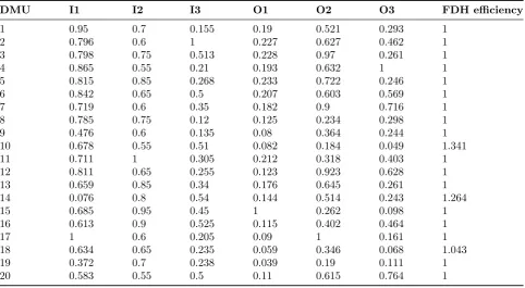
Table 1: The data for 20 Iranian bank branches.
DMU I1 I2 I3 O1 O2 O3 FDH efficiency
1 0.95 0.7 0.155 0.19 0.521 0.293 1
2 0.796 0.6 1 0.227 0.627 0.462 1
3 0.798 0.75 0.513 0.228 0.97 0.261 1
4 0.865 0.55 0.21 0.193 0.632 1 1
5 0.815 0.85 0.268 0.233 0.722 0.246 1
6 0.842 0.65 0.5 0.207 0.603 0.569 1
7 0.719 0.6 0.35 0.182 0.9 0.716 1
8 0.785 0.75 0.12 0.125 0.234 0.298 1
9 0.476 0.6 0.135 0.08 0.364 0.244 1
10 0.678 0.55 0.51 0.082 0.184 0.049 1.341
11 0.711 1 0.305 0.212 0.318 0.403 1
12 0.811 0.65 0.255 0.123 0.923 0.628 1
13 0.659 0.85 0.34 0.176 0.645 0.261 1
14 0.076 0.8 0.54 0.144 0.514 0.243 1.264
15 0.685 0.95 0.45 1 0.262 0.098 1
16 0.613 0.9 0.525 0.115 0.402 0.464 1
17 1 0.6 0.205 0.09 1 0.161 1
18 0.634 0.65 0.235 0.059 0.346 0.068 1.043
19 0.372 0.7 0.238 0.039 0.19 0.111 1
20 0.583 0.55 0.5 0.11 0.615 0.764 1
Figure 1: Illustration of marginal rates of substi-tution in FDH.
4
Empirical Example
To apply the proposed method on real data, we employ the above mentioned method and algo-rithm on the empirical example used in [11] and [13]. As it can be seen in Table 1, the data set consists of 20 DMUs with 3 inputs and 3 outputs. The data are originally reported by Amirteimoori et al. [13] which consist of 20 Iranian bank branches or DMUs in 2005. The three outputs include deposits, loans and charges. The three in-puts include staff, computer terminals and space. In Table 2, we can see the results of the output-oriented FDH model. It can be found that
thir-teen bank branches are efficient (All units are ef-ficient except for DMUs 10, 14 and 18).
Based on model (3.5), for example, if the staff of DM U13 increases with 0.1, the marginal rate of substitution from the right between staff and deposits is 0.60. In other words, increasing Staff with 0.1, results in increasing deposits with 0.06. Also to the left, which is when staff decreases with 0.1, it results in increasing deposit with 0.96. As another example, if the staff of DM U3 increases with 0.1, the marginal rate of substitution from the right between staff and deposits is 0.05. In other words, increasing staff with 0.1, results in increasing deposits with 0.05. Also to the left, which is when staff decreases with 0.1, it results in increasing Deposit with 1.48. These results are compiled in Table2.
5
Conclusion
trade-T
able
2:
Staff
and
Dep
osit
marginal
rates
of
substitution
for
h
=
0
.
1
,h
′=
−
0
.
1
D
M
U
1
2
3
4
5
6
7
8
9
10
11
12
13
14
15
16
17
18
19
20
M
R
S
+ x1 y1
0.03
0
0.05
0
0
0.21
0
0.68
0
-0
0.7
0.06
-0
0.97
1.03
-0
0
M
R
S
− x1 y1
i.f
i.f
1.48
i.f
1.53
i.f
i.f
i.f
i.f
-1.32
i.f
0.96
-1.32
0.35
i.f
-i.f
i.f
offs between staff and deposit in twenty branches of an Iranian bank for efficient units.
Acknowledgements
Financial support by Lahijan Branch, Islamic Azad University Grant No. 1235, 17-20-5/3507 is gratefully acknowledged.
References
[1] P. J. Agrell, J. Tind, A Dual Approach to Nonconvex Frontier Models,Journal of
Pro-ductivity Analysis 16 (2001) 129-147.
[2] A. R. Amirteimoori, S. Kordrostami, Effi-cient surfaces and an efficiency index in DEA : a constant returns to scale,Applied
Mathe-matics and computation 163 (2005) 683-691.
[3] M. Asmild, J. C. Paradi, D. N. Reese, The-oretical perspectives of trade-off analysis us-ing DEA,Omega 34 (2006) 337-343.
[4] W. W. Cooper, K. S. Park, J. T. Pastor Ciurana, Marginal rates and elasticities of substitution with additive models in DEA,
Journal of productivity Analysis 13 (2000)
105-123.
[5] F. R. Frsund, L. Hialmarsson, Are all scales optimal in DEA? Theory and empirical ev-idence, Journal of Productivity Analysis 21 (2004) 25-48.
[6] Z. Huang, S. X. Li, J. J. Rousseau, De-termining rates of change in data envelop-ment analysis, Journal of the Operational
Research Society 48 (1997) 591-593.
[7] M. Izadikhah, A Step by Step Method to Im-prove the Performance of Decision Making Units, Journal of mathematical Extension 9 (2015) 91-107.
[9] L. Khoshandam, R. K. Matin, A. Amirteimoori, MRS in DEA with un-desirable outputs: A directional approach,
Measurement 68 (2015) 49-57.
[10] A. Masoumzadeh, M. Toloo, A. Amirteimoori, Performance assessment in production systems without explicit inputs: an application to basketball players,
IMA Journal of Management Mathematics
27 (2016) 143-156.
[11] M. Mirzaei, S. Kordrostami, A. Amirteimoori, M. G. Chegini, Hindawi Pub-lishing Corporation, Article ID 1531282, (2016).
[12] D. Rosen, C. Schaffnit, J. C. Paradi, Marginal rates and two dimensional level curve in DEA,Journal of productivity Anal-ysis 9 (1998) 205-232.
[13] A. Zanella, Ana S. Camanho, Teresa G. Dias, Undesirable output and weighting schemes in composite indicators based on DEA,
Eu-ropean Journal of Operational Research 245
(2015) 1-14.
Mohsen Mirzaei is a PhD candidate at the department of applied mathematics, Lahijan branch, Islamic Azad University. His research interests include op-erations research and data envel-opment analysis.
Sohrab Kordrostami is a full professor in applied mathematics (operations research field) depart-ment in Islamic Azad University, Lahijan branch. He completed his Ph.D. degree in Islamic Azad University of Tehran, Iran. His research interests include performance manage-ment with special emphasis on the quantitative
methods of performance measurement, and espe-cially those based on the broad set of methods known as Data Envelopment Analysis, (DEA). Kordrostami’s papers have appeared in a wide se-ries of journals such as Applied mathematics and computation, International journal of advanced manufacturing technology, etc.
Alireza Amirteimoori is a full professor in applied mathematics operations research group in Is-lamic Azad University in Iran. He completed his Ph. D degree in Is-lamic Azad University in Tehran, Iran. His research interests lie in the broad area of performance management with special emphasis on the quantitative methods of performance measurement, and especially those based on the broad set of methods known as Data Envelopment Analysis, (DEA). Amirteimoori’s papers appear in journals such as Applied math-ematics and computation, Journal of the oper-ations research society of Japan, International Journal of Production Economics and etc.