INTELIGENCIA ARTIFICIAL
http://journal.iberamia.org/
Hybrid Adaptive Computational Intelligence-based
Multisensor Data Fusion applied to real-time UAV
autonomous navigation
ˆ
Angelo de Carvalho Paulino
[1,2,A], Lamartine Nogueira Frutuoso Guimar˜
aes
[2,B], Elcio
Hideiti Shiguemori
[2,C][1]
ITA - Aeronautics Institute of Technology, S˜ao Jos´e dos Campos – 12.228-900, Brazil.
[2]
IEAv - Institute for Advanced Studies, S˜ao Jos´e dos Campos – 12.228-001, Brazil.
[A]
[email protected],[B][email protected],[C][email protected]
AbstractNowadays, there is a remarkable world trend in employing UAVs and drones for diverse applications. The main reasons are that they may cost fractions of manned aircraft and avoid the exposure of human lives to risks. Nevertheless, they depend on positioning systems that may be vulnerable. Therefore, it is necessary to ensure that these systems are as accurate as possible, aiming to improve navigation. In pursuit of this end, conventional Data Fusion techniques can be employed. However, its computational cost may be prohibitive due to the low payload of some UAVs. This paper proposes a low-cost Multisensor Data Fusion application based on Hybrid Adaptive Computational Intelligence (HACI) - the cascaded use of Fuzzy C-Means Clustering (FCM) and Adaptive-Network-Based Fuzzy Inference System (ANFIS) algorithms - that have been shown able to improve considerably the accuracy of current positioning estimation systems for real-time UAV autonomous navigation, reducing the error in approximately 300cm2. In addition, the proposed methodology outperformed two other Computational Intelligence methodologies – Artificial Neural Networks and Regression Models, with 18 different tested approaches – in estimating an UAV position considering the Root-Mean-Square Error against the real trajectory. The generated Fuzzy Inference System has proved to be effective in providing an improved positioning estimation with a low computational burden, about 600 times faster than the fastest embedded sensor refresh rate.
Keywords: Data Fusion, Computational Intelligence, Unmanned Aerial Vehicles, Autonomous Navigation, In-ertial Sensors, Positioning Estimation, ANFIS.
1
Introduction
Several applications are possible for aerospace assets. Among them, one can mention the integration and logistics for different sectors of the society, the assessment of natural or public calamities, and the moni-toring of areas of government interest [1]–[3]. Manned aircraft with onboard remote sensing equipment, such as cameras, sensors, and radars, have been responsible for detailed tracking, data collecting and help in detecting threats, aiming at protecting and upholding the law [4]–[9].
However, for many applications, the use of manned aircraft is not feasible or desirable since the crew lives may be exposed to risk scenarios, like situations involving disasters or radiation. In many cases, this could be avoided. Therefore, an alternative to the use of manned aircraft is the use of Unmanned
ISSN: 1137-3601 (print), 1988-3064 (on-line) c
Aerial Vehicles (UAVs) [9], [10]. Given some factors like their low flying altitude and slow speed, they are more difficult to be detected by conventional sensors [9]. In addition, some models cost only a fraction of manned aircraft. According to Cook [9], the UAVs, which historically were thought of as merely complementary to manned aircraft, have proven to be an excellent power asymmetry tool.
The world trend in the use of UAVs is undeniable. The use of such systems in the military plays an important role in surveillance, reconnaissance, target prediction, and even combat missions by operating in a wider range of conditions and scenarios than conventional aircrafts [9]–[12]. Regarding the civilian scope of aerospace robotics employment, there can be mentioned topographic surveys, mapping of areas of interest, precision agriculture, surveillance, and access control, remote sensing for geological and cli-matic research and various utilities [2], [3], [8], [12]. State-of-the-art applications include detection and monitoring of sea wildlife [13], thermographic inspection of photovoltaic plants [15], radiation detection [14] and identification of helicopter landing zones and airdrop zones in calamity situations [16].
Though, it is known that UAVs require a structured navigation control protocol, such as via Radio Frequency or via satellite, which makes it vulnerable to interference such as jamming or spoofing [10]. One solution to this problem is the use of autonomous navigation. However, even the use of Global Navigation Satellite Systems (GNSS) or Inertial Navigation System (INS) - systems widely covered in the literature - are not immune to faults or interference [17]. Ignoring the attitude and trajectory of an aircraft can cause the loss of the aircraft altogether, so it is essential to ensure the operational reliability, accuracy, and robustness of their navigation [8].
In this sense, the use of Data Fusion to enable more secure and robust navigation is a good alternative to the exclusive reliance on the usual navigation systems. The technology of Data Fusion plays an invaluable role in the search for increased navigational safety [23, 18]. Therefore, given the reality of the current applications of aerospace robotics, promoting research and development in the area of Data Fusion is imperative [1], [8], [12].
Thus, the main objective of this paper is to evaluate a Multisensor Data Fusion application, based on Hybrid Adaptive Computational Intelligence (HACI), through the fusion and integration of sensed data obtained by embedded sensors of the UAVs. The proposed approach aims to reduce the imprecision of current methods of positioning estimation, like GPS and INS, and to deliver solutions in a feasible time to the problem of real-time navigation of low-performance UAVs. The proposed methodology offers an improvement in the quality of the positioning estimation information provided as input to its In-flight Navigation and Attitude Control System – a system responsible for controlling the UAV’s frame attitude and trajectory and for the Decision-Making process – or simply “control loop”. It is hoped, therefore, to provide UAVs with safer and more robust navigation given more precise information is being used for the flight. It should be noted that the control loop modeling is not in the scope of this article.
The referred Fusion has been performed using two Computational Intelligence techniques in a cascaded way, i.e., Fuzzy C-Means Clustering (FCM) [60] and Adaptive-Network-Based Fuzzy Inference System (ANFIS) [61]. These techniques have shown to be promising to effectively increase the accuracy of the positioning estimation of the UAV held by the Global Positioning System (GPS), considering the Root-Mean-Square Error (RMSE) between the position taken as real and the estimated one. The methodology proposed in this work was compared with two other Computational Intelligence methodologies – Artificial Neural Networks and Regression Models – with 18 different tested approaches, outperforming them in the capability of enhancing the positioning estimation precision considering the RMSE against the real trajectory, as detailed in the next sections.
2
Data Fusion and related work
The systems most widely employed for the navigation of UAVs are the GNSS. The most known are the GPS and the Globalnaya Navigatsionnaya Sputnikovaya Sistema (GLONASS) [8], [17], [19]. Nonetheless, several studies show that these systems may present vulnerabilities, both from natural factors, such as the South Atlantic Magnetic Anomaly (SAMA), and human factors, such as jamming, spoofing and malicious blockages and interference [21]–[26].
multiple sensors for the positioning estimation has shown to be a feasible option to the dependence on one or the other system alone [27]–[29].
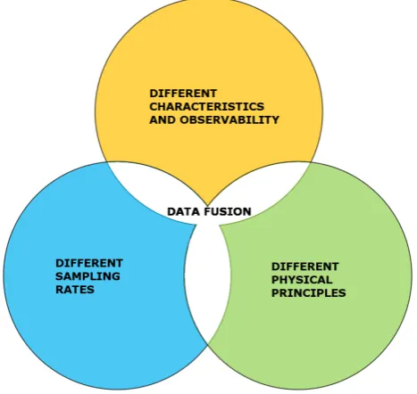
Along with technological development, the number of available sensors and data has been increasing. In general, it is seen that there is a need to use different sources of data to obtain more accurate estimates [8, 24]. In this context, Data Fusion techniques can be used to fuse the data originated from various sensors and thereby generate improved information [23, 24]. Figure 1 shows possible combinations of differences between data sources.
Figure 1: Possible combinations of differences between data sources addressed by Data Fusion.
In the literature, several recent works deal with the improvement of the positioning estimation using Data Fusion of GPS and INS. The positioning estimation is done through different methods, as seen, for instance, in [30]-[34], where is shown the fusion of GPS and INS to bridge the period of GPS outages for vehicular navigation. The authors in [35] use random forest regression to enhance the positioning estimation of an airplane, whereas [40] employs Kalman filtering to a high-performance ultra-tightly coupled GPS/INS. In [36]-[39] is seen the use of adaptive networks to perform the Multisensor Data Fusion. Additionally, [41, 42] apply Fuzzy Inference Systems to perform the fusion. Finally, it is seen in [43] the use of ANFIS as a sub-remedy system to temporarily replace the GPS positioning estimation used as input to a Kalman filter during GPS outages. Although, according to the authors, the methodology implies an average performance improvement of not more than 40%, the great counterpoint to this work is that the employed methodology is subject to all the problems related to the use of the Kalman filter. Problems include imprecision about noise information that could lead to position and velocity deviations and filter divergences due to system linearization, which implies in no guarantee of optimality [45, 48, 44]. The Data Fusion approach has shown to be effective in reducing the imprecision of the positioning estimation process. Nevertheless, it is worth mentioning that the only papers found regarding the im-provement of the autonomous navigation of a UAV using ANFIS as the main estimator was published by the authors in [46] and [47].
With that said, Data Fusion is a process that acts through the detection, association, correlation, estimation and combination of data of different sensors [18], [48], [49]. This may be invaluable for the collection of useful information aiming at the analysis of the various scenarios for Decision-Making [50]. Regarding UAVs, the higher the exposure to an unfamiliar and unstructured scenario, the higher the risk in its operation due to eventual obstacles that may arise in its trajectory [10].
com-bination in an optimized way, acquiring statistical advantages by increasing the number of observations of the same event; improvement of the observation process using relative data between multiple sensors, which opens up new possibilities for combining and extracting information; and greater observability, since a sensor can capture data that another cannot, either by divergences in their physical nature, position or refresh rate, for example, reducing errors and complementing information [12], [48].
However, the use of several sensors can imply large volumes of data, sometimes noisy, with different characteristics, unconjugated sampling rates or even nature and physical principles that are de-correlated with each other. Therefore, considering the complexity of such a data set, conventional Data Fusion techniques may not present timely solutions to the navigation problem, given, in general, its high com-putational cost [48], [50], and also considering the need for real-time processing in the case of an ongoing flight.
Hence, a Data Fusion application based on HACI is proposed, aiming at making feasible its employ-ment in real-time flight applied to the problem of navigation, given the mathematical simplicity of the tool used to estimate the position [51] and its inherent low computational cost.
3
FCM and ANFIS
The tool used to perform the Data Fusion was the Fuzzy logic, which is the representation of uncertainties in the mathematical form [53]. Regarding aerospace systems, the uncertainties arise mainly from their complexity and non-linearity, both as a result of inaccuracies in the mathematical model and the number of variables that interact epistatically in obtaining the results [70]. In the field of multivalued logic, it is important to emphasize that this logic, considered as of “infinite” values, aims to formalize the representation of vagueness using linguistic terms [54]. Thus, it is an efficient solution to the fusion of vague, noisy or partial data [50].
Focusing on the applications, Fuzzy logic is extremely flexible for the most diverse uses since it uses “membership functions” (MFs) that model and quantify the meaning of the symbols [50, 70] for their deductive apparatus in an intuitive and close to the natural language way [54], through well-defined “if-then” relationship rules [70]. A good example of the application of Fuzzy logic is its use to improve the accuracy of the landing procedure of an UAV [38]. Another is the joint use with Computational Vision tools for estimating the position of an UAV in real-time flight, based on landmark recognition, as seen in [52].
Fuzzy logic fits into the Soft Computing area, which refers to the use of computational tools to find approximate solutions to approximately formulated problems, creating some tolerance for imprecision and uncertainties aiming at modeling systems in a more treatable, robust and cost-effective way, with greater computational power saving and communication bandwidth [70]. Thus, Soft Computing is a good choice for the implementation of intelligent control of complex systems, such as aerospace systems. Other areas of Artificial Intelligence are also covered by Soft-Computing, among them: Artificial Neural Networks, Probabilistic Reasoning, Expert Systems, and Genetic Algorithms [70].
In the case of neural networks, Kothari and Bhattacharjee [56] state that it is a stochastic and heuristic tool that learns the relation between the parameters and their responses when trained with a finite number of input data and predicts the values of a new set of independent variables based on their training (learning) experience. It should be noted that, from the optimization point of view, “learning” is equivalent to minimize the global error function [58]. With that said, neural networks are interesting because they can handle some complex problems through a powerful and flexible framework [59].
According to Teodorovi´c [57], the chosen structure of a neural network model can influence the con-vergence rate of a training algorithm and even determine the type of learning to be used. Also according to the author, the training algorithms are very simple mechanisms that adapt the weights of the branches of a network, requiring for each node only locally available data. For this reason, he concludes that its implementation generally does not involve complex calculations and, thereby, powerful computational configurations are not necessary. For this work, the chosen architecture was the Multi-Layer Perceptron (PMC), one of the most used in the literature [55].
second one is an Adaptive Network – a class of feed-forward Neural Networks with supervised learning capability – that emulates the behavior of a Fuzzy Inference System (FIS) System [61].
In the case of a flight data (log) containing real data captured from embedded sensors, such as the one used in this work, there is a significant amount available for extracting information. This is a task that is not trivial [62]. Consequently, techniques that use methods that combine knowledge areas such as machine learning, pattern recognition, and information retrieval can be employed towards a better analysis of the data [62].
3.1
The Fuzzy C-Means Clustering (FCM) algorithm
Like any clustering technique, the FCM assists in obtaining an intuition about data whose volume makes the analysis by humans difficult. For this reason, algorithms such as FCM are widely used for exploratory data analysis in the sense that they act as meta-learning tools [62].
According to Saxena et al. [63], clustering techniques can be divided into Hierarchical, such as BIRCH, CURE, ROCK, and CHAMELEON, or Partitional, such ask-means, PAM, CLARA, CLARANS, FCM, EM, DBSCAN, and CLICK. As stated in [64], clustering techniques can be divided, according to the sta-tistical point of view, into a probabilistic approach, based on a model that uses probability distributions, or in a non-parametric approach, which essentially employs methods based on objective functions of sim-ilarity or dissimsim-ilarity. Also according to Yang and Nataliani [64], the best-known probabilistic algorithm is the Expectation-Maximization (EM), while thek-means is the most famous among the non-parametric. Another example of a non-parametric algorithm is the FCM, used in this work.
Crisp clustering algorithms consider that each sample may belong to one, and only one centroid. This prevails in the fact that such algorithms present difficulties in modeling systems that exhibit uncertainties of non-statistical nature, such as noises [60]. Thus, the Fuzzy Set Theory proves to be substantially useful since it formalizes the mathematical representation of vagueness/uncertainty [65], which can be applied to the clustering problem.
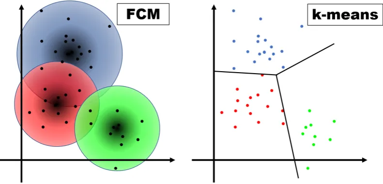
Unlike crisp clustering techniques, such ask-means andx-means, the FCM allows one sample to belong to a greater or lesser degree to more than one centroid, determined by a Fuzzy membership function [63]. This expands both the ability of differentiation and of agglomeration between samples and allows, for example, the identification of noises in regions of overlapping membership [60]. A simple illustration of the fact is depicted in Figure 2.
Figure 2: Simplified representation on how FCM andk-means algorithms cluster the data.
Jm= N X i=1 c X j=1
umijkxi−vjk2; 1< m <∞ (1)
whereN is the number of samples,cthe number of centroids,ma real number that controls the degree of overlap between the centroids, uij(Fuzzy Partition Matrix) the level at which an observationxi belongs to a cluster j, vj the j-th cluster’s centroid, andk ∗ k represents any norm that expresses the similarity between the measured data and the centroids, such as the Euclidian norm in (1).
Thus, the FCM algorithm is comprised of the following steps [60], [63], [66]:
1. The initial values of theuij membership functions of the centroids (c) are randomly adjusted;
2. Calculate the prototype centroids (j = 1, ... ,c):
Vj=
PN
i=1u m ijxi
PN
i=1umij
(2)
3. Calculateuijaccording to:
uij =
" c
X
k=1
kxi−vjk
kxi−vkk
m2−1#
−1
(3)
4. Calculate Objective FunctionJm (1); and
5. Repeat steps 2 to 4 untilJm reaches the desired convergence or the iteration number exceeds a stipulated limit.
In this paper, the centroids calculated by the FCM algorithm are then used as the starting point for the generation of initial membership functions that will be optimized by the ANFIS algorithm.
3.2
The Adaptive-Network-Based Fuzzy Inference System (ANFIS)
algo-rithm
The ANFIS algorithm, developed by Jang [61], uses a hybrid learning scheme and can construct an input-output type mapping based on human knowledge, represented by if-then rules and associated pairs of inputs and outputs. In this sense, it is able to learn to map highly nonlinear functions [61], [67]. Briefly, this algorithm can be seen as a flexible mathematical structure that can address the approximation of a large class of complex nonlinear systems with a desirable level of accuracy [67], without, however, losing the mathematical rigor [51], [65].
Concerning the Fuzzy Logic, it should be emphasized that there is no standard methodology for transforming human knowledge or experience into a rule base for a FIS. In addition, there is a need to make adjustments to the established membership functions to both improving performance and minimizing systems’ errors [61]. Hence, finding appropriate rules and applying appropriate adjustment methods are key issues [68], and the adequate representation of these rules is crucial.
Thus, the form of treatment of if-then rules proposed by Takagi and Sugeno (T-S) is particularly inter-esting since it employs parameters of mathematical functions in place of the classic linguistic expressions [51], [68] and has fuzzy sets involved only in the part of the premises [61]. Here is an example of T-S type fuzzy reasoning:
Rule1 :IF x is A1 AN D y is B1, T HEN f1=p1x+ q1y+r1
Rule2 :IF x is A2 AN D y is B2, T HEN f2=p2x+ q2y+r2
In this approach, the consequent part is described by non-fuzzy equations of fuzzy input variables (antecedents) [61]. This particular fact allows its application in several machine learning algorithms, among which is the ANFIS algorithm.
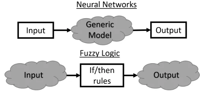
By using a hybrid scheme of Fuzzy Logic and Neural Networks such as Adaptive Networks, an ANFIS Network harnesses advantages of these two large areas of Computational Intelligence [69]. While Fuzzy Logic can handle uncertainty in inputs and outputs, Adaptive Networks can address the uncertainty of the model and thus, when employed synergistically, can be applied to a wide variety of complex problems [70]. Figure 3 illustrates the complementarity of these two paradigms.
Figure 3: Neural Networks and Fuzzy Logic and how they deal with uncertainty (clouds).
The complementarity depicted in Figure 3 is achieved by means of an Adaptive Network structure, according to Figure 4 [61], [71]:
Figure 4: Structural model of an ANFIS Network. The arrows indicate the direction of the hybrid learning scheme. Source: Adapted from [71].
Each layer of the structure has the following constitution:
1. Fuzzy sets that determine the degree of membership of inputsxandy : µAi(x) andµBi(y) .
3. Normalization of activations, according to:
wi= w1w+wi 2 (4)
4. Defuzzification according to consequent’s parameterspi ,qi andri .
5. Output as a function of the sum of activation of all the rules (composition):
f =P
iwifi=
P iwifi P
iwi (5)
Once the structure of the Adaptive Network was detailed, the steps of the ANFIS algorithm applied to the context of this work are as follows:
1. Load thetraining andvalidation data and determine the input parameters and number of epochs;
2. Generate initial membership functions (antecedents);
3. Perform the training of the ANFIS System by means of a hybrid optimization of the FIS model (Figure 4) until a predetermined stop criterion is reached (maximum error, for example):
(a) Antecedents: Fixed in the forward pass (forth) of the algorithm and optimized in the backward pass (back) by the Gradient Descent method, based on the outputs of the model; and
(b) Consequents: Optimized on the forward pass (forth) by the Least Square Optimization (LSE), based on error rates (e), and fixed at the backward pass (back)
4. Validate training results - trained ANFIS systems - according tovalidation data; and
5. Verify the efficiency of the trained model by measuring the degree of accuracy of the model in predicting the output, given certain inputs, through RMSE.
The use of the ANFIS Networks proposed in this work is performed with real data obtained in flight as explained below. Several configurations were tested for four dimensions, namely: number of inputs (sensors used); number of membership functions for each input; number of training epochs; and data division for training. The results are discussed in section 5.
4
Materials and methods
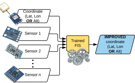
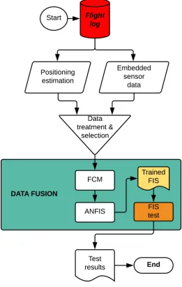
The methodology chosen for this scientific work - which is now detailed - promotes the Data Fusion through HACI, using real measured data of several embedded sensors from flight logs. These logs were generated in real-time. Once the data is presented, the chosen algorithms perform a non-linear mapping from the input data (coordinate and chosen sensors) to the output data (real position), generating trained Fuzzy Inference Systems. The trained FIS are then used to perform the positioning estimation of the UAV, as shown in Figure 5. Several tests presented at section 5 show the evaluation of the proposed methodology effectiveness.
The Real-Time Kinetic GPS sensor data, treated by a Kalman filter (KF-GPS-RTK), was used as ground truth. Given its notorious precision, this data makes it possible to measure the errors of the positioning estimates generated by the Data Fusion System. It should be noted that the dataset of a flight log refers to all samples taken between takeoff and landing with a given sampling rate.
According to Al-Hmouzet al [71], the choice of training data is of paramount importance. However, given the complexity of data such as those recorded in flight logs of an UAV, choosing the training, validation, andgeneralizationdata sets that provide the best results is not trivial. Thus, Cross-Validation (CV) techniques can be employed to minimize the risk - or error - in the choice of data groups, bearing in mind that the data groups are chosen in order to be independent of each other [73].
Figure 5: Illustration of the methodology applied to the improvement of the positioning estimation of a UAV using Hybrid Adaptive Computational Intelligence.
presented data. According to Varoquaux [74], CV is the best tool available in this assignment, since it is the only nonparametric method for the generalization capability test. Therefore, once the ANFIS Networks trained in this work are aimed at the real-time flights, it is hoped that such capacity will be as high as possible.
The chosen technique was a modified version of theK-fold Cross-Validation (KFCV), which, in ad-dition to presenting a mild computational cost, divides the data into K sub-samples of approximately equal cardinality [76, 73]. This way, each sub-sample successively exerts the role of the validation set [73] and generalization set, when present. The common use of cross-validation techniques considers a set ofK−1 sub-samples for training and 1 for validation. The modification proposed in this work consists that nowK−2 sub-samples are used for the training set, 1 is used for the validation set, and another 1 sub-sample is used for the generalization set.
In the literature, optimal values forK are commonly chosen between 5 and 10 [74], [75]. However, a small number of samples may imply bad results [74]. Considering that in the literature it is commonly seen that something about 70% to 80% of data is used for training, the number 7 was chosen for theK value since the training set will have 5/7 of the sub-samples, or about 71,4% of the data being used as training set as well. With that said, the chosen technique will be henceforth called 7FCV in this work.
The whole dataset was permutated, and the data samples assigned to each sub-sample randomly taken. Then 5 of the 7 sub-samples are chosen to compose the training set; 1 to the validation set; and 1 to the generalization set. This way,C7
5∗C12(42) independent combinations (groups) of the 7 sub-samples were generated for the application of the proposed methodology, numbered from 1 to 42. The 7FCV data division scheme is used only from the fourth series of experiments and on, once the first three series of experiments have their own peculiarities regarding the data division, as demonstrated in section 5.
4.1
Methodology phases
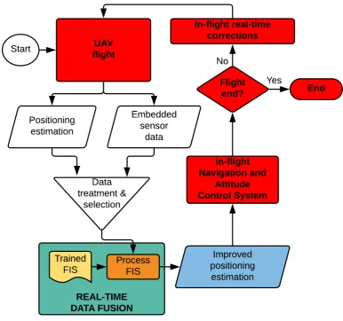
latter, the data can be presented in real-time flight or simulated flight time, in the case of previous flights (logs). Regarding previous flights, it is assumed that the next position to be provided for the Data Fusion System has already been duly corrected by the In-flight Navigation and Attitude Control System. The flowcharts of each phase are shown in Figures 6 and 7. It is stated, however, that the red items in the flowcharts are outside the scope of this study and, therefore, will not be detailed.
4.1.1 Training phase
The training phase (Figure 6) aims to generate a FIS that can be used for the Data Fusion positioning estimation once new data is presented to it. Thus, the flight log will provide the dataset to be used for the training, which includes the data of all embedded sensors. Hence, sensor data such as GPS estimates are taken to provide the estimated positions at each instant of time. KF-GPS-RTK sensor data supplies the true position and other sensors data that will be used for the fusion are taken as well. The data is loaded in batches that correspond to the entire flight time, from takeoff to landing.
Then the cross-validation scheme 7FCV is responsible - when present - for generating the 42 combina-tions of the 7 different sub-samples at this time. After that, the data is presented to the FCM algorithm for the initial FIS creation. For the FCM stage, the degree of centroid overlapping (m) was empirically adjusted at about 1.2 for the significant majority of the tests. The initial FIS generated by the FCM algorithm is then optimized by the ANFIS algorithm, beaconed by the validation sub-sample. Once trained, the FIS is subjected to efficiency and efficacy tests in the positioning estimation of an UAV -generally with the generalization sub-sample data. The results are then recorded for performance control and eventual re-use. This ends the training phase.
4.1.2 Employment phase
The employment phase (Figure 7) intends to apply the FIS trained in the previous phase in a real or simulated flight, in order to improve the accuracy of positioning estimation of an UAV. Thus, from the point at which a flying UAV generates positioning and embedded sensors data, such data is processed and selected. It is worth mentioning that, unlike the training phase, where the data is loaded in batches, in the case of real-time use the data is processed timely at each given instant of time. Then, the chosen data is provided as input to the trained FIS to perform the Data Fusion, as seen in Figure 5, where a more accurate positioning estimate is obtained.
The improved positioning estimation is then used to feed in the In-flight Navigation and Attitude Control System. Such a system - which will not be treated within the scope of this Work - will carry out the necessary corrections in real flight time and will feedback the shown flowchart given the flight end was not reached. Thereafter, the UAV flight follows normally with a corrected positioning estimation at each new iteration until landing.
Once the proposed methodology is shown, the details of the flight data used for practical experimen-tation will be explored.
4.2
WITAS Dataset
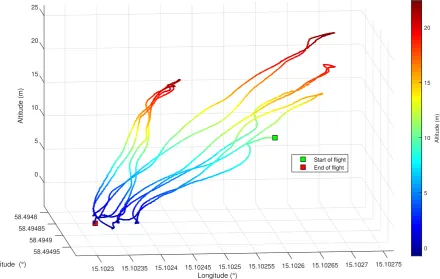
A flight was performed by the WITAS Project [72] in an area centered at the coordinates 58◦29’ 41.58.6” N and 15◦06’ 09.0” E, in Sweden. The UAV used is based on the commercial model “Yamaha Rmax UAV”, equipped with avionics developed at the Department of Computer & Information Science - Link¨oping University [72].
In Figure 8 the flight path of the UAV is presented, recorded with a Real-Time Kinetic GPS and refined by a Kalman Filter (KF-GPS-RTK), with sub-meter accuracy. The path was recorded in three dimensions: Latitude, Longitude, and Altitude. The scale to the right of the graph reflects the Altitude values, in order to make it easier to understand the graph. The starting and endpoints are shown as well.
0 5 10 15 20 25 Altitude (m) 58.4948 58.49485
Latitude (°) 58.4949 58.49495 Longitude (°) 15.10275 15.1027 15.10265 15.1026 15.10255 15.1025 15.10245 15.1024 15.10235 15.1023 0 5 10 15 20 Altitude (m)
Start of flight End of flight
Figure 8: Trajectory of the flight performed by the WITAS Project UAV.
The UAV avionics has captured 139 different types of real-time flight data, including data from embedded sensors such as compass, barometer, GPS, and INS (Accelerometer and Gyroscope), among others. For this work, the data listed in Table 1 were extracted.
Table 1: Data used in this work.
SENSOR REFRESH RATE EXTRACTED DATA NO. OF VARIABLES
Embedded GPS 10 Hz
Clock, Latitude (GPS-Lat) and Longitude (GPS-Lon) 4 Embedded Accelerometer (ACCEL)
66 Hz Acceleration fields - X,
Y and Z axis 4
Embedded Gyroscope
(GYRO) 200 Hz
Angular rates relative to Euler angles (Roll, Pitch and Yaw rates)
4
KF-GPS-RTK 50 Hz
Reference/truth for both Latitude and
Longitude
3
Table 2: Detail of data use according to each series of experiment.
SERIES NO. QTY. OF
SAMPLES
INTERPOLATED
DATA 7FCV NO. OF TESTS
1 66,483 Yes No 4
2 66,483 Yes No 6
3 66,483 Yes No 100
4 66,483 Yes Yes 336
5 3,319 No Yes 672
6 3,319 No Yes 225
Table 2 shows how the data has been used in the experiments series, indicating whether the 7FCV scheme was employed or not. In addition, the table indicates the number of tests of each series, the number of samples considered for training and if the data was interpolated or not. It’s worth mentioning that the 7FCV scheme was not employed at the 3 first series because the main purpose of these series was to gather information about the general functionalities of the FCM+ANFIS methodology and its interactions with the flight log data.
5
Experiments and results
In this work, experiments were carried out with different architectures of the ANFIS Network to assess the effectiveness of the methods studied in this work. Five series were carried out, totaling more than 1,115 different tests. These experiments initially aimed at a better understanding of the data set and also the way how ANFIS work, to then evaluate the possible improvement in the accuracy of the positioning estimation by embedded sensors. In the experiments, tests were performed by varying the four dimensions mentioned before, to gather intuitions about the behavior of the ANFIS Network in each configuration.
A final series was held aiming at the testing of two other Data Fusion methodologies, namely Ar-tificial Neural Networks (ANNs) and Regression Models (RM), totaling more than 255 tests. Different approaches for both methodologies were tested. For the ANNs, the chosen training approaches were Levenberg-Marquardt [81], Bayesian Regularization [80] and Scaled Conjugate Gradient [79]. As for the RMs, 15 training approaches of four different classes were tested [82]-[87]: for Linear Regressions class, Linear, Interactions Linear, Robust Linear, and Stepwise Linear; for the Trees class, Fine Tree, Medium Tree and Coarse Tree; for the Support Vector Machines class, Linear SVM, Quadratic SVM, Cubic SVM, Fine Gaussian SVM, Medium Gaussian SVM and Coarse Gaussian SVM; and finally, for the Ensembles class, Boosted Trees and Bagged Trees. The sixth series was performed for the sake of comparison with the results obtained by the FIS trained by the ANFIS algorithm.
notorious accuracy, either for Latitude or for Longitude. Therefore, in relation to KF-GPS-RTK, it was measured that embedded GPS presents an RMSE of approximately 21.10cm in Latitude and 30.81cm in Longitude.
Regarding the number of training epochs, some considerations have to be made. The algorithm used is instructed to generate two FIS: one at the end of the set number of epochs; and another which produced the least error among all epochs, or best fitness, if not equal to the first FIS. Although the number of epochs is fixed, the shown results correspond to the least error value found during the training process, that not necessarily corresponds to the last epoch of training. This fact is not a problem since the fuzzy inference system that yielded the best results of the entire training process will ever be available for the next experiments. The information about which epoch corresponds to the best result of a given test is not relevant to this work.
The experiments were performed on a notebook PC with a Core [email protected] processor, 16GB RAM, and a 64 bit Windows 10 Operating System.
5.1
First experiment series - the influence of the number of training epochs
A first approach was performed to preliminarily assess the impact of the number of training epochs on the performance of the technique. It is well known that an insufficient number of epochs may not promote the necessary convergence, whereas a large number of epochs may lead to overfitting [71].
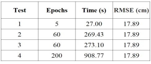
Having fixed the quantities of 2 input membership functions and a training set of 80% of the data, the number of training epochs was varied for GPS-Lat and ACCEL sensors in 4 tests. The results are shown in Table 3.
Table 3: Results for the first series – 2 sensors.
From the analysis of Table 3 it is seen that increasing the number of training epochs did not imply a significant improvement in the performance of the trained network. The computational time, in turn, was severely affected, indicating that increasing the number of training epochs is not always advantageous.
5.2
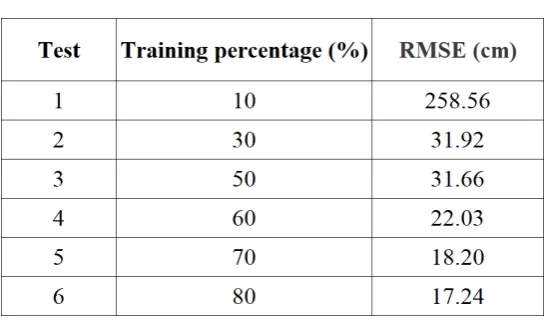
Second experiment series - the influence of training percentage
Given the preliminary results regarding the influence of the number of epochs on the achieved result, a series was performed to understand the influence of the percentage of the data used for the training. It is commonly seen in the literature the use of high percentages of the data for the training of Adaptive Networks.
Table 4: Results for the second series – 3 sensors.
From these experiments, it was confirmed that the higher the percentage of data used for training, the better the overall performance of the trained network. The different tested data percentages were 10% , 30% , 50% , 60% , 70% and 80% . Furthermore, it was observed that using data from three sensors, GPS-Lat, ACCEL, and GYRO, showed better results than using only GPS-Lat and ACCEL, when comparing the last result of Table 4 with those of Table 3.
5.3
Third experiment series - the influence of the number of membership
functions
Knowing minimally satisfactory parameters for conducting new tests, the third series was performed. The purpose of this study was to evaluate the impact of the number of membership functions per input to be optimized by the ANFIS algorithm in the performance of the proposed technique. For this purpose, the percentage of 70% of the data for the training was adopted, considering the good performance presented in the previous series.
In this series of 100 tests, the fused sensors were GPS-Lat and ACCEL, an association that presented relevant results. Both the number of MFs per input (2, 3, 4 e 5 MFs) and the number of epochs (5, 10, 50, 100 and 500 epochs) were combined and tested. For each of the 20 combinations of MFs per input and epochs, the generalization capability was evaluated by the average of 10 repetitions of the evaluation of 10,000 points randomly taken from the whole dataset.
Unlike the previous series, here the coordinates are not considered as inputs. That is, the input variables of the FIS refer only to the other sensors, which are mapped to the difference between the position estimated by the KF-GPS-RTK and that provided by the embedded GPS. The motivation arose from the perception that including the coordinates as inputs, besides increasing the processing time, demand that the direct employment (with no offset) of the FIS is restricted to the window of the coordinates used for training. This is due to the fact that the maximum and minimum values of each input variable are used to establish the FIS Universes of Discourse.
Therefore, the strategy of not treating coordinates as inputs — but as a difference — is interesting in the sense that performing non-linear mapping for a difference, rather than for an absolute value, makes its application feasible in regions of flight not used for training. It should be noted that, since the proposed approach concerns only the coordinate, its effectiveness is likely to be greater on flights with similar conditions, albeit in different regions. That is, issues such as trajectory, velocity, and similar climatic characteristics are factors that should bring positive contributions to the performance of the Data Fusion. Thus,∆ corresponds to the horizontal inaccuracy of the UAV in degrees. A mathematical representation~ for determining the difference to be used for training can be found in the Equation 4.
~
∆ =pos~ out−pos~ in (4)
example in a new flight, a position estimated by a GPS could be improved by a trained FIS with the calculation that appears in Equation 5:
~
pos0out=pos~ 0in+∆ +~ ~e∆ (5)
with the vectorpos~ 0out representing the improved position and pos~ 0inthe input coordinate estimated by the GPS, the∆ is obtained by the Data Fusion promoted by the trained FIS and the vector~ ~e∆represents the model error. Such an error is unknown a priori and composes the positioning estimation.
In short, the significant advantage of the strategy used is that both the location of the flight and the dimensions of the coordinate window used for training are no longer limiting factors for the employment of the methodology. However, the study of the impact of all other factors besides the coordinates, such as changes in speed, trajectory, and climatic characteristics, is suggested as future work. Thus, the results obtained are shown in Figure 9.
(a) Average by number of epochs
(b) Average by number of rules
Confirming the hypothesis about the results obtained previously for this dataset, it was seen that increasing the number of training epochs in many cases proved to be ineffective in the generalization results, in relation to the RMSE mean. Also, increasing the number of MFs per input indistinctly has led to a worsening of the results, except for the leap from 2 to 3 MFs per input. Finally, the best results were achieved with a 5 epoch and 3 MFs per input setting, as seen in Figure 9. However, the use of 2 MFs per input enables a performance comparable to 3 MFs per input, but with shorter processing time. This fact prevailed in the choice of 2 MFs per input for the next series.
5.4
Fourth experiment series - the influence of the data organization
The fourth series was undertaken with the main purpose of evaluating the impact of data organization on the performance of the proposed methodology. The values of 5 epochs and 2n rules were adopted, where 2 is the number of MFs per input and n is the number of input sensors. This variable amount of rules aims to provide more structural complexity to networks that will handle increased sets of data, from the addition of data inputs from other sensors. In other words, more sensors used imply more rules appearing in the structures of the ANFIS networks. Thus, 168 tests were performed for GPS-Lat associated with other sensors, and other 168 similar tests for GPS-Lon. Also, from this series onwards, the dataset employed was structured according to the 7FCV Cross-Validation technique.
In this series was observed that, indeed, the choice of CV groups combinations exerted great influence on the performance of ANFIS Networks. As an example, in the fusion of 3 sensors (GPS-Lon, ACCEL, and GYRO), the worst combination (no18) showed an error 73.40% greater than the best combination (no10). The RMSE comparison of the performance of each CVtraining groups in predicting the corresponding validation groups is showed in Figure 10. Additionally, it was seen that the average computational time went from 8.52s (2 rules) to 9.225s (8 rules), until remarkable 644.12s for 64 rules, with worse results, worth mentioning.
Concerning Figure 10, the bars indicate the concentration of the second quartile results for each CV group, with the upper and lower limits indicating, respectively, the delimitation of the third and first quartiles. The “whiskers” indicate the extremes that are not considered outliers. Red and green squares indicate respectively the best performance in terms of minimum and average of the whole set of tests, for a given coordinate. Finally, the “target” present in each bar indicates the median of the results for each CV group and the triangles down and up an indication about the significance of the differences between the medians.
Through an analysis of the tables of results and a visual inspection of these graphs, the choice of the training data has shown to have a great impact on the performance of the methodology. Furthermore, it was seen that there is a certain tendency that groups that perform well for GPS-Lat perform as good as for GPS-Lon. The best results were achieved with the CV combination no10, that yielded the following results: 17.38cm for GPS-Lat + ACCEL fusion and 24.86cm for GPS-Lon + ACCEL + GYRO fusion, both results better than the embedded GPS estimation alone. As for the worst results, they are 26.27cm for GPS-Lat + ACCEL + GYRO and 43.11cm for GPS-Lon + ACCEL + GYRO.
5.5
Fifth experiment series - the impact of using coordinates as inputs
In order to obtain better results and, primarily, to compare the performance of strategies that consider or not the coordinate as input, this fifth series was undertaken. Thanks to good results obtained previously, the values of 50 epochs and 16 rules were adopted for all the 672 tests.
1 2 3 4 5 6 7 8 9 10 11 12 13 14 15 16 17 18 19 20 21 22 23 24 25 26 27 28 29 30 31 32 33 34 35 36 37 38 39 40 41 42
CV group number
16 17 18 19 20 21 22 23 24 25 26
Latitude estimation error (cm)
Minimum value Minimum average
(a) Latitude
1 2 3 4 5 6 7 8 9 10 11 12 13 14 15 16 17 18 19 20 21 22 23 24 25 26 27 28 29 30 31 32 33 34 35 36 37 38 39 40 41 42
CV group number
20 25 30 35 40
Longitude estimation error (cm)
Minimum value Minimum average
(b) Longitude
(a) ∆-Latitude
(b) Latitude
(a) ∆-Longitude
(b) Longitude
Figure 12: Performance measured in terms of RMSE (cm) of each CV training group based on the prediction capability for the generalization group, for each combination of sensors - Longitude and ∆-Longitude - fifth series.
The results show that the performance of the networks that consider the coordinates as inputs was slightly better than those considered “∆-coordinate”. However, the latter can be applied quickly on a broader range of scenarios because they do not use absolute values. Also, was seen that using data from all available sensors does not always bring improvements to the performance of networks, but results indicate that, for the given data set, fusing data from two or more sensors is advantageous. The summary of the best results obtained in the Fifth series is in Table 5.
(a) FIS model
(b) FIS rules
(a) FIS model
(b) FIS rules
(a) Latitude
(b) Longitude
Table 5: Comparison of best positioning estimation RMSE according to each combination of the different sensors, regarding each of the base coordinates.
5.6
Sixth experiment series - comparison with other methods and final results
In this last series, the fusion was performed using ANNs and RMs, tuned with well-known parameters, in 225 tests, aiming at a comparison with the now fine-tuned FCM+ANFIS. The ANNs were trained with a two-layer feed-forward architecture with sigmoid hidden neurons and linear output neurons. The input layer is composed of 4 neurons for both Latitude and Longitude since the best results were obtained with 2 sensors (GPS-Lat/Lon + ACCEL, with ACCEL having 3 variables). The hidden layer has 2,000 neurons and the output just one, the improved coordinate estimate. A data division was performed, where 70% of the samples were used for training, 15% for validation and 15% for testing, with samples taken randomly. The training process had no fixed epoch number, being halted when the generalization capability stopped improving. Finally, the best results were 17.02cm for Latitude and 24.70cm for Longitude. For the ANNs, the training algorithm that yielded the best results was the Bayesian Regularization. Table 7 at the appendix lists the best results for each training method.
Regarding the RMs, the best results were obtained with 3 sensors for Latitude (GPS-Lat + ACCEL + GYRO) and 2 for Longitude (GPS-Lon + ACCEL), trained with Interactions Linear and Fine Tree techniques respectively. All tests were performed with a 7-fold Cross-Validation scheme over the sample data. It is worth mentioning that the Fine Tree was employed with a minimum leaf size of 4 and maximum surrogates per node of 10. The best obtained results were 19.15cm for Lat and 24.34cm forLon. Table 8 at the appendix presents the best results for each approach.
Based on the estimates of Latitude and Longitude performed by the FIS trained by ANFIS Networks, a comparison can be made with the estimates made by the GPS, the ANNs and the RMs through the evaluation of their respective RMSE, which is shown in Table 6. An excerpt of the trajectories estimated by each Fusion method, the real trajectory provided by the KF-GPS-RTK and the trajectory estimated by the embedded GPS is shown in Figures 16 and 17, as well as the comparison of error between the methods’ estimates and the truth trajectory for the given coordinate. It is appropriate to mention that the figures include only short excerpts of such trajectories and that at other regions of the complete plot the other methods were eventually more precise than the trained ANFIS algorithm.
(a) Complete trajectory - Latitude
(b) Detailed trajectory - instants 742 to 805
(c) Detailed trajectory error - instants 742 to 805
(a) Complete trajectory - Longitude
(b) Detailed trajectory - instants 2530 to 2610
(c) Detailed trajectory error - instants 2530 to 2610
In general, all approaches prevailed in an imprecision reduction of the positioning estimation. After a thorough visual inspection of the trajectories (Figures 16 and 17) estimated by the algorithms, it was perceived that the estimates made by all the fusion methods have some sensitivity to input signal noise. Such sensitivity can be easily seen in Figure 18, which allows immediate identification of the tendency of the points estimated by the various methods to follow the original noisy signal (blue line). Due to the complexity of the data of a real flight log, in the excerpts where noises are present, the estimates diverge significantly from the actual trajectory. In other words, the proposed methodology showed some sensitivity to noises tending to follow the GPS’s quick variation noises, indicating that prior treatment of GPS deviations would bring improvements to the methodology employment. In addition, noises regarding other sensors might influence the outliers present in excerpts where the blue line shows low variation. The analysis of all these facts is suggested as future work. Finally, it was observed that the overall performance of the ANFIS Systems exceeded by 45.19% the accuracy of the estimation performed by the GPS.
2640 2660 2680 2700 2720 2740
Temporal sequence of the samples 58.494942 58.494944 58.494946 58.494948 58.49495 58.494952 58.494954 58.494956 58.494958 58.49496 58.494962 Latitude (°) Embedded GPS KF-GPS-RTK (Reference) FCM+ANFIS ANN RM (a) Latitude
3220 3240 3260 3280 3300 3320
Temporal sequence of the samples 15.102305 15.10231 15.102315 15.10232 Longitude (°) Embedded GPS KF-GPS-RTK (Reference) FCM+ANFIS ANN RM (b) Longitude
5.7
Final remarks
Although no tests of the FIS fusion were conducted on actual UAVs – but on a notebook PC – it was found that, for a total of 3,319 estimates by fusing the sensors corresponding to the best trained FIS for each coordinate, the average time of 100 repetitions of the 3,319 estimates was 2.0317s for Lat and 2.7081s for Lon, or about 6.12 x 10⁻⁶ and 8.16 x 10⁶ seconds per estimation, respectively. This fact reveals that, indeed, a FIS is of high-speed processing, considering the computational power of the used notebook PC, with updates occurring at more than 120,000 estimates per second (∼= 163kHz -Lat e∼= 122kHz - Lon). A feature like this is of great interest in the application of the developed methodology to real-time navigation. Tests on real-time flights with the FIS fusion being performed by the embedded avionics of an UAV are suggested as future work.
6
Conclusions
As demonstrated in the results of the carried-out experiments, the methodology employed in this Mul-tisensor Data Fusion application, using a HACI methodology, has shown to be effective in increasing the positioning estimation precision. In the tests, the technique presented a reduction of approximately 300cm2 in the area error, compared to the estimation of the position provided by the embedded GPS. How useful this reduction is, in practice, depends on the selected application. Applications that need high precision could be undoubtedly benefited. In addition, the proposed methodology outperformed two other Computational Intelligence methodologies, with 18 different approaches. The obtained results show that the use of multiple data sources has brought benefits to the solution of the navigation problem, considering the safety in the operation of the UAV, by offering less uncertainty to the Decision-Making System.
The main contribution of this work is the development of a Data Fusion application which presents a desirable level of accuracy and a low computational cost. This can make feasible its use in real-time autonomous navigation by low-performance UAVs, considering they usually lack computational power and payload. Once trained, the T-S rules-based FIS system has shown to be indeed agile, considering the computer used in the tests, to perform positioning estimation based on multidimensional data, about 600 times faster than the fastest sensor refresh rate. However, given the complexity of a flight log, further analysis of the trained fuzzy rules didn’t bring any new useful knowledge, as expected.
Although the good performance, the proposed methodology still shows some sensitivity to noise in some parts of the trajectory. An assessment of the impact of noise treatment or reduction is suggested as future work since it could, theoretically, improve the performance of the employed techniques. In addition, at this point of the research, there is no guarantee that the proposed methodology will present comparable performance in flights with completely different trajectories or weather conditions. Studies in this sense are proposed as future work as well.
Other suggestions for future work include: perform the fusion with sensors other than GPS and INS; a study of why the other methods were more precise than ANFIS in some particular excerpts of the trajectory; perform the fusion using other Computational Intelligence Data Fusion methodology, and the conduction of tests on new flights data.
References
[1] BRASIL. Minist´erio da Defesa. Comando da Aeron´autica. Planejamento., DCA 11-45 - Concep¸c˜ao Estrat´egica For¸ca A´erea 100. 2014.
[2] M. G. Lacerda, ˆA. C. Paulino, ´A. J. Dami˜ao, E. H. Shiguemori, and Lamartine N. F. Guimar˜aes, “O Emprego de ´Arvore de Decis˜ao para a Identifica¸c˜ao e Classifica¸c˜ao de ZLs e ZPHs em Imagens Obtidas por ARPs de Pequeno Porte”, in XIX Simp´osio de Aplica¸c˜oes Operacionais em ´Areas de Defesa, 2017.
Zones and Airdrop Zones in Calamity Situations”, in ICUAS 2018: International Conference on Unmanned Aircraft Systems, 2018, vol. 12, no. 5, p. 2190.
[4] Agˆencia For¸ca A´erea, “Veja o trabalho dos esquadr˜oes especializados em reconhecimento a´ereo”, 2017. [Online]. Available: www.fab.mil.br/noticias/mostra/30328. [Accessed: 21-Feb-2018].
[5] Agˆencia For¸ca A´erea, “Hermes 900 participa de treinamento em Campo Grande”, 2014. [Online]. Available: http://fab.mil.br/noticias/mostra/19863. [Accessed: 17-Feb-2018].
[6] Agˆencia For¸ca A´erea, “Esquadr˜ao H´orus participa da vigilˆancia a´erea nos Jogos Ol´ımpicos”, 2016. [Online]. Available: http://fab.mil.br/noticias/mostra/26951. [Accessed: 17-Feb-2018].
[7] Agˆencia For¸ca A´erea, “FAB intercepta aeronave que transportava 500 kg de droga”, 2017. [Online]. Available: www.fab.mil.br/noticias/mostra/30439. [Accessed: 21-Feb-2018].
[8] A. Al-Kaff, D. Mart´ın, F. Garc´ıa, A. de la Escalera, and J. Mar´ıa Armingol, “Survey of computer vision algorithms and applications for unmanned aerial vehicles”, Expert Syst. Appl., vol. 92, pp. 447–463, Feb. 2018. doi: 10.1016/j.eswa.2017.09.033.
[9] K. L. B. Cook, “The Silent Force Multiplier: The History and Role of UAVs in Warfare”, in 2007 IEEE Aerospace Conference, 2007, pp. 1–7. doi: 10.1109/AERO.2007.352737.
[10] L. Davis, M. J. McNerney, J. Chow, T. Hamilton, S. Harting, and D. Byman, “Armed and Danger-ous? UAVs and U.S. Security”, Santa Monica, CA, 2014.
[11] D. Glade, “Unmanned Aerial Vehicles: Implications for Military Operations”, Occas. Pap. Cent. Strateg. Technol. Air War Coll., no. 16, p. 38, 2000.
[12] M. E. Liggins, D. L. Hall, and J. Llinas, Handbook of multisensor data fusion: theory and practice, 2nd ed. Boca Raton, FL: CRC Press, 2009.
[13] U. K. Verfuss et al., “A review of unmanned vehicles for the detection and mon-itoring of marine fauna,” Mar. Pollut. Bull., vol. 140, pp. 17–29, Mar. 2019. doi: 10.1016/J.MARPOLBUL.2019.01.009.
[14] C. M. Chen, L. E. Sinclair, R. Fortin, M. Coyle, and C. Samson, “In-flight performance of the Ad-vanced Radiation Detector for UAV Operations (ARDUO),” Nucl. Instruments Methods Phys. Res. Sect. A Accel. Spectrometers, Detect. Assoc. Equip., Nov. 2018. doi: 10.1016/J.NIMA.2018.11.068.
[15] S. Gallardo-Saavedra, L. Hern´andez-Callejo, and O. Duque-Perez, “Technological review of the in-strumentation used in aerial thermographic inspection of photovoltaic plants,” Renew. Sustain. En-ergy Rev., vol. 93, pp. 566–579, Oct. 2018. doi: 10.1016/J.RSER.2018.05.027.
[16] M. G. Lacerda, A. De Carvalho Paulino, E. H. Shiguemori, A. J. Damiao, L. N. F. Guimaraes, and C. S. dos Anjos, “Identification and Classification of Drop Zones and Helicopter Landing Zones in Images Obtained by Small Size Remotely Piloted Aircraft Systems,” in IGARSS 2018 -2018 IEEE International Geoscience and Remote Sensing Symposium, -2018, pp. 7906–7909. doi: 10.1109/IGARSS.2018.8517753.
[17] W. da Silva, “Navega¸c˜ao Autˆonoma de VANT em per´ıodo noturno com imagens Infravermelho Termal”, INPE, 2016.
[18] R. Cardoso, “Integra¸c˜ao de Sensores Via Filtro de Kalman”, ITA, 2003.
[19] W. da Silva, E. H. Shiguemori, N. L. Vijaykumar, and H. F. de C. Velho, “Estimation of UAV position with use of thermal infrared images”, in 2015 9th International Conference on Sensing Technology (ICST), 2015, pp. 828–833. doi: 10.1109/ICSensT.2015.7438511.
[21] G. Conte and P. Doherty, “An Integrated UAV Navigation System Based on Aerial Image Matching”, in 2008 IEEE Aerospace Conference, 2008, pp. 1–10. doi: 10.1109/AERO.2008.4526556.
[22] L. Faria, C. M. Silvestre, and M. A. F. Correia, “GPS-Dependent Systems: Vulnerabilities to Elec-tromagnetic Attacks”, J. Aerosp. Technol. Manag., vol. 8, pp. 423–430, 2016.
[23] J. R. G. Braga, “Navega¸c˜ao autˆonoma de VANT por imagens LiDAR,” Instituto Nacional de Pesquisas Espaciais, 2018.
[24] P. F. F. Silva Filho, “Automatic Landmark Recognition in aerial images for the autonomous naviga-tion system of Unmanned Aerial Vehicles”, ITA, 2016.
[25] L. D. A. Faria, C. A. de M. Silvestre, M. A. F. Correia, and N. A. Roso, “GPS Jamming Signals Propagation in Free-Space, Urban and Suburban Environments”, J. Aerosp. Technol. Manag., vol. 10, pp. 1–8, Feb. 2018. doi: 10.5028/jatm.v10.870.
[26] L. D. A. Faria, C. A. de M. Silvestre, M. A. F. Correia, and N. A. Roso, “Susceptibility of GPS-Dependent Complex Systems to Spoofing”, J. Aerosp. Technol. Manag., vol. 10, pp. 1–11, Jan. 2018. doi: 10.5028/jatm.v10.839.
[27] G. Stamatescu, I. Stamatescu, D. Popescu, and C. Mateescu, “Sensor fusion method for altitude esti-mation in mini-UAV applications”, in 2015 7th International Conference on Electronics, Computers and Artificial Intelligence (ECAI), 2015, p. SSS-39-SSS-42. doi: 10.1109/ECAI.2015.7301203.
[28] S.-M. Oh, “Multisensor fusion for autonomous UAV navigation based on the Unscented Kalman Filter with Sequential Measurement Updates”, in 2010 IEEE Conference on Multisensor Fusion and Integration, 2010, pp. 217–222. doi: 10.1109/MFI.2010.5604461.
[29] C. Luo, S. I. McClean, G. Parr, L. Teacy, and R. De Nardi, “UAV Position Estimation and Collision Avoidance Using the Extended Kalman Filter”, IEEE Trans. Veh. Technol., vol. 62, no. 6, pp. 2749–2762, Jul. 2013. doi: 10.1109/TVT.2013.2243480.
[30] J. Li, N. Song, G. Yang, M. Li, and Q. Cai, “Improving positioning accuracy of vehicular navigation system during GPS outages utilizing ensemble learning algorithm”, Inf. Fusion, vol. 35, pp. 1–10, 2017. doi: 10.1016/j.inffus.2016.08.001.
[31] S. Adusumilli, D. Bhatt, H. Wang, V. Devabhaktuni, and P. Bhattacharya, “A novel hybrid approach utilizing principal component regression and random forest regression to bridge the period of GPS outages”, Neurocomputing, vol. 166, pp. 185–192, Oct. 2015. doi: 10.1016/J.NEUCOM.2015.03.080.
[32] A. Noureldin, A. El-Shafie, and M. Reda Taha, “Optimizing neuro-fuzzy modules for data fusion of vehicular navigation systems using temporal cross-validation”, Eng. Appl. Artif. Intell., vol. 20, no. 1, pp. 49–61, Feb. 2007. doi: 10.1016/J.ENGAPPAI.2006.03.002.
[33] D. Bhatt, P. Aggarwal, V. Devabhaktuni, and P. Bhattacharya, “A novel hybrid fusion algorithm to bridge the period of GPS outages using low-cost INS”, Expert Syst. Appl., vol. 41, no. 5, pp. 2166–2173, 2014. doi: 10.1016/j.eswa.2013.09.015.
[34] X. Li, W. Chen, C. Chan, B. Li, and X. Song, “Multi-sensor fusion methodology for enhanced land vehicle positioning”, Inf. Fusion, vol. 46, pp. 51–62, Mar. 2019. doi: 10.1016/J.INFFUS.2018.04.006.
[35] S. Adusumilli, D. Bhatt, H. Wang, P. Bhattacharya, and V. Devabhaktuni, “A low-cost INS/GPS integration methodology based on random forest regression”, Expert Syst. Appl., vol. 40, no. 11, pp. 4653–4659, 2013. doi: 10.1016/j.eswa.2013.02.002.
[37] N. Musavi and J. Keighobadi, “Adaptive fuzzy neuro-observer applied to low cost INS/GPS”, Appl. Soft Comput., vol. 29, pp. 82–94, Apr. 2015. doi: 10.1016/J.ASOC.2014.12.024.
[38] M. K. Al-Sharman, B. J. Emran, M. A. Jaradat, H. Najjaran, R. Al-Husari, and Y. Zweiri, “Precision landing using an adaptive fuzzy multi-sensor data fusion architecture”, Appl. Soft Comput., vol. 69, pp. 149–164, Aug. 2018. doi: 10.1016/J.ASOC.2018.04.025.
[39] A. Noureldin, A. El-Shafie, and N. El-Sheimy, “Adaptive neuro-fuzzy module for inertial navigation system/global positioning system integration utilising position and velocity updates with real-time cross-validatio”,. doi: 10.1049/iet-rsn:20070001.
[40] S. H. Oh and D.-H. Hwang, “Low-cost and high performance ultra-tightly coupled GPS/INS in-tegrated navigation method”, Adv. Sp. Res., vol. 60, no. 12, pp. 2691–2706, Dec. 2017. doi: 10.1016/J.ASR.2017.06.007.
[41] H. Nourmohammadi and J. Keighobadi, “Fuzzy adaptive integration scheme for low-cost SINS/GPS navigation system”, Mech. Syst. Signal Process., vol. 99, pp. 434–449, Jan. 2018. doi: 10.1016/J.YMSSP.2017.06.030.
[42] V. Havyarimana, D. Hanyurwimfura, P. Nsengiyumva, and Z. Xiao, “A novel hybrid approach based-SRG model for vehicle position prediction in multi-GPS outage conditions”, Inf. Fusion, vol. 41, pp. 1–8, May 2018. doi: 10.1016/J.INFFUS.2017.07.002.
[43] C. H. Lim, T. S. Lim, and V. C. Koo, “Implementation of ANFIS for GPS-aided INS UAV motion sensing at short term GPS outage,” J. Comput. Sci., vol. 10, no. 12, pp. 2564–2575, Dec. 2014. doi: 10.3844/jcssp.2014.2564.2575.
[44] K. Saadeddin, M. F. Abdel-Hafez, M. A. Jaradat, and M. A. Jarrah, “Optimization of Intelligent Approach for Low-Cost INS/GPS Navigation System,” J. Intell. Robot. Syst., vol. 73, no. 1–4, pp. 325–348, Jan. 2014. doi: 10.1007/s10846-013-9943-2.
[45] X. Wang and W. Wang, “Nonlinear Signal-Correction Observer and Application to UAV Navigation,” IEEE Trans. Ind. Electron., vol. 66, no. 6, pp. 4600–4607, Jun. 2019. doi: 10.1109/TIE.2018.2860540.
[46] ˆA. de C. Paulino, L. N. F. Guimar˜aes, and E. H. Shiguemori, “An Adaptive Neuro-Fuzzy-based Mul-tisensor Data Fusion applied to real-time UAV autonomous navigation,” in ENIAC 2018 - Encontro Nacional de Inteligˆencia Artificial e Computacional, 2018, pp. 847–858. doi: 10.5753/eniac.2018.4472.
[47] G. da P. Neto, ˆA. de C. Paulino, E. H. Shiguemori, H. F. de C. Velho, and L. N. F. Guimar˜aes, “Computational Intelligence-based Multisensor Data Fusion applied to positioning estimation and autonomous navigation of an UAV,” in Conference of Computational Interdisciplinary Science 2019, 2019, pp. 1–13.
[48] F. Castanedo, “A Review of Data Fusion Techniques”, Sci. World J., vol. 2013, pp. 1–19, 2013. doi: 10.1155/2013/704504.
[49] F. E. White, “Data Fusion Lexicon”, Jt. Dir. Lab. Tech. Panel C3, Data Fusion Sub-Panel, Nav. Ocean Syst. Cent., p. 16, 1991.
[50] B. Khaleghi, A. Khamis, F. O. Karray, and S. N. Razavi, “Multisensor data fusion: A review of the state-of-the-art”, Information Fusion, vol. 14, no. 1. Elsevier, pp. 28–44, 01-Jan-2013. doi: 10.1016/j.inffus.2011.08.001.
[51] T. Takagi and M. Sugeno, “Fuzzy Identification of Systems and Its Applications to Modeling and Control”, IEEE Trans. Syst. Man Cybern., vol. SMC-15, no. 1, pp. 116–132, 1985. doi: 10.1109/TSMC.1985.6313399.
[53] T. J. Ross, Fuzzy logic with engineering applications, 3rd ed., vol. 761. West Sussex: John Wiley & Sons Ltd, 2010.
[54] Y. Tanaka, “An overview of fuzzy logic,” in WESCON/’93. Conference Record, 1993, pp. 446–450. doi: 10.1109/WESCON.1993.488475.
[55] W. Mao and F.-Y. Wang, “Cultural Modeling for Behavior Analysis and Prediction,” in Advances in Intelligence and Security Informatics, Elsevier, 2012, pp. 91–102. doi: 10.1016/B978-0-12-397200-2.00008-7.
[56] V. K. Kothari and D. Bhattacharjee, “Artificial neural network modelling for prediction of thermal transmission properties of woven fabrics,” in Soft Computing in Textile Engineering, Elsevier, 2011, pp. 403–423. doi: 10.1533/9780857090812.5.403.
[57] D. Teodorovi´c, “Traffic and Transportation Analysis Techniques,” in Transportation Engineering, Elsevier, 2017, pp. 63–162. doi: 10.1016/B978-0-12-803818-5.00003-2.
[58] M. F. Møller, “A scaled conjugate gradient algorithm for fast supervised learning,” Neural Networks, vol. 6, no. 4, pp. 525–533, Jan. 1993. doi: 10.1016/S0893-6080(05)80056-5.
[59] S. K. Das, “Artificial Neural Networks in Geotechnical Engineering,” in Metaheuristics in Wa-ter, Geotechnical and Transport Engineering, Elsevier, 2013, pp. 231–270. doi: 10.1016/B978-0-12-398296-4.00010-6.
[60] J. C. Bezdek, R. Ehrlich, and W. Full, “FCM: The fuzzy c-means clustering algorithm”, Comput. Geosci., vol. 10, no. 2, pp. 191–203, 1984. doi: 10.1016/0098-3004(84)90020-7.
[61] J.-S. R. Jang, “ANFIS: adaptive-network-based fuzzy inference system”, IEEE Trans. Syst. Man. Cybern., vol. 23, no. 3, pp. 665–685, 1993. doi: 10.1109/21.256541.
[62] P. Nerurkar, A. Shirke, M. Chandane, and S. Bhirud, “Empirical Analysis of Data Clustering Algorithms”, Procedia Comput. Sci., vol. 125, pp. 770–779, Jan. 2018. doi: 10.1016/J.PROCS.2017.12.099.
[63] A. Saxena et al., “A review of clustering techniques and developments”, Neurocomputing, vol. 267, pp. 664–681, Dec. 2017. doi: 10.1016/J.NEUCOM.2017.06.053.
[64] M.-S. Yang and Y. Nataliani, “Robust-learning fuzzy c-means clustering algorithm with unknown number of clusters”, Pattern Recognit., vol. 71, pp. 45–59, Nov. 2017. doi: 10.1016/J.PATCOG.2017.05.017.
[65] L. A. Zadeh, “Fuzzy sets”, Inf. Control, vol. 8, no. 3, pp. 338–353, 1965. doi: 10.1016/S0019-9958(65)90241-X.
[66] The MathWorks Inc., “FCM”, 2018. [Online]. Available: https://www.mathworks.com/help/fuzzy/fcm.html. [Accessed: 24-May-2018].
[67] S. Kamarian, M. H. Yas, A. Pourasghar, and M. Daghagh, “Application of firefly algorithm and ANFIS for optimisation of functionally graded beams”, J. Exp. Theor. Artif. Intell., vol. 26, no. 2, pp. 197–209, 2014. doi: 10.1080/0952813X.2013.813978.
[68] H. Zamani Sabzi, D. Humberson, S. Abudu, and J. P. King, “Optimization of adaptive fuzzy logic controller using novel combined evolutionary algorithms, and its application in Diez Lagos flood controlling system, Southern New Mexico”, Expert Syst. Appl., vol. 43, pp. 154–164, Jan. 2016. doi: 10.1016/J.ESWA.2015.08.043.
[70] L. H. Tsoukalas and R. E. Uhrig, Fuzzy and Neural Approaches in Engineering, 1st ed. New York, NY, USA: John Wiley & Sons, Inc., 1997.
[71] A. Al-Hmouz, Jun Shen, R. Al-Hmouz, and Jun Yan, “Modeling and Simulation of an Adaptive Neuro-Fuzzy Inference System (ANFIS) for Mobile Learning”, IEEE Trans. Learn. Technol., vol. 5, no. 3, pp. 226–237, 2012. doi: 10.1109/TLT.2011.36.
[72] G. Conte and P. Doherty, “Vision-Based Unmanned Aerial Vehicle Navigation Using Geo-Referenced Information”, EURASIP J. Adv. Signal Process., vol. 2009, no. 1, p. 387308, Dec. 2009. doi: 10.1155/2009/387308.
[73] S. Arlot and A. Celisse, “A survey of cross-validation procedures for model selection”, Stat. Surv., vol. 4, pp. 40–79, 2010. doi: 10.1214/09-SS054.
[74] G. Varoquaux, “Cross-validation failure: Small sample sizes lead to large error bars”, Neuroimage, Jun. 2017. doi: 10.1016/J.NEUROIMAGE.2017.06.061.
[75] Y. Zhang and Y. Yang, “Cross-validation for selecting a model selection procedure”, J. Econom., vol. 187, no. 1, pp. 95–112, 2015. doi: 10.1016/j.jeconom.2015.02.006.
[76] C. Bergmeir, R. J. Hyndman, and B. Koo, “A note on the validity of cross-validation for evaluating autoregressive time series prediction,” Comput. Stat. Data Anal., vol. 120, pp. 70–83, 2018. doi: 10.1016/j.csda.2017.11.003.
[77] L. Xu et al., “Stochastic cross validation,” Chemom. Intell. Lab. Syst., vol. 175, pp. 74–81, Apr. 2018. doi: 10.1016/J.CHEMOLAB.2018.02.008.
[78] T. T. Wong, “Performance evaluation of classification algorithms by k-fold and leave-one-out cross validation,” Pattern Recognit., vol. 48, no. 9, pp. 2839–2846, Sep. 2015. doi: 10.1016/j.patcog.2015.03.009.
[79] S. Berisha and J. G. Nagy, “Iterative Methods for Image Restoration,” in Academic Press Library in Signal Processing, vol. 4, Elsevier, 2014, pp. 193–247. DOI: 10.1016/B978-0-12-396501-1.00007-8.
[80] Z. Sun, Y. Chen, X. Li, X. Qin, and H. Wang, “A Bayesian regularized artificial neural net-work for adaptive optics forecasting,” Opt. Commun., vol. 382, pp. 519–527, Jan. 2017. DOI: 10.1016/J.OPTCOM.2016.08.035.
[81] A. Sharif Ahmadian, “Numerical Methods and Procedures,” in Numerical Models for Submerged Breakwaters, Elsevier, 2016, pp. 93–108. DOI: 10.1016/B978-0-12-802413-3.00006-7.
[82] G. M. Fitzmaurice, “Regression,” Diagnostic Histopathol., vol. 22, no. 7, pp. 271–278, Jul. 2016. DOI: 10.1016/j.mpdhp.2016.06.004.
[83] M. Fern´andez-Delgado, M. S. Sirsat, E. Cernadas, S. Alawadi, S. Barro, and M. Febrero-Bande, “An extensive experimental survey of regression methods,” Neural Networks, vol. 111, pp. 11–34, Mar. 2019. DOI: 10.1016/J.NEUNET.2018.12.010.
[84] B. Choubin, E. Moradi, M. Golshan, J. Adamowski, F. Sajedi-Hosseini, and A. Mosavi, “An ensemble prediction of flood susceptibility using multivariate discriminant analysis, classification and regression trees, and support vector machines,” Sci. Total Environ., vol. 651, pp. 2087–2096, Feb. 2019. DOI: 10.1016/J.SCITOTENV.2018.10.064.
[85] A. Nazarpour, G. R. Paydar, and E. J. M. Carranza, “Stepwise regression for recognition of geo-chemical anomalies: Case study in Takab area, NW Iran,” J. Geogeo-chemical Explor., vol. 168, pp. 150–162, Sep. 2016. DOI: 10.1016/J.GEXPLO.2016.07.003.
[86] I. The MathWorks, “Choose Regression Model Options,” 2019. [Online]. Available: https://www.mathworks.com/help/stats/choose-regression-model-options.html. [Accessed: 11-Mar-2019].
Appendix
See tables 7 and 8.
Table 7: Best results for each training method - ANNs.