R E S E A R C H A R T I C L E
Open Access
Partitioned simulation strategies for
fluid–structure–control interaction
problems by Gauss–Seidel formulations
Andreas Winterstein
1*, Christopher Lerch
2, Kai-Uwe Bletzinger
1and Roland Wüchner
1*Correspondence:
1Chair of Structural Analysis,
Technical University of Munich, Arcisstraße 21, 80333 Munich, Germany
Full list of author information is available at the end of the article
Abstract
In this contribution the multi-physics problem of fluid–structure–control interaction (FSCI) is solved by an iterative, partitioned approach utilizing Gauss–Seidel
formulations. The aim is to conduct a fully coupled co-simulation of the FSCI problem, where the controller actively influences the dynamics of the structure. The purpose of this manuscript is twofold: In the first part, in order to get a profound idea of the behavior and parametric sensitivity of such systems involving multiple couplings, the simplified model problem introduced for fluid–structure interaction (FSI) by Joosten, Dettmer and Peri´c is extended by a generic control unit. Since a monolithic solution for this simplified model problem can be found, it is used for first investigations
concerning solvability and stability. On this basis, three different variants for coupling the subsystems fluid, structure and controller by a Gauss–Seidel scheme, are derived and systematically investigated. More precisely the FSCI problem is solved without nesting of the subsystems in the first variant and with nesting of two of the respective subsystems in the second and third variant. In the second part, the resulting algorithms are applied to a complex, non-linear, multi-degree of freedom problem, which is a well-known benchmark problem in the FSI community and is therefore extended to FSCI. Applying those algorithms to the multi-degree of freedom problem shows good results and substantiates the applicability to such problems. It follows, actively influencing the dynamics of the structure in the FSCI problem by a controller reduces the structural vibrations induced by the fluid flow significantly.
Keywords: Fluid–structure interaction, Multi-physics, State-feedback control, Partitioned solution procedure, Fluid–structure–control interaction (FSCI), Co-simulation
Introduction
The development in the community of coupled problems tends more and more to deal-ing with multi-physics problems containdeal-ing more than two physical fields. One of the first contributions for the partitioned treatment of such problems has been made in [1], which gives a general overview about the treatment of coupled problems by a par-titioned approach. More recent developments are for example fluid–structure interac-tion with electro magnetics [2], fluid–structure–contact interaction [3] or general n-field coupling [4,5].
©The Author(s) 2018. This article is distributed under the terms of the Creative Commons Attribution 4.0 International License (http://creativecommons.org/licenses/by/4.0/), which permits unrestricted use, distribution, and reproduction in any medium, provided you give appropriate credit to the original author(s) and the source, provide a link to the Creative Commons license, and indicate if changes were made.
In this contribution the coupled problem of fluid–structure–control interaction (FSCI) is treated in a partitioned way. This means a closed-loop control unit, which manipulates the dynamics of the structure, is added to the well-known two field problem of fluid– structure interaction (FSI). This kind of problem statement was first mentioned in [1, p. 3262 and 3263], but has not been followed in more detail. Also in [4], FSCI to reduce flow induced structural displacements has been mentioned as a side note in the context of testing the algorithm developed therein. In contrast to the present contribution, a rigid structure with one degree of freedom with small displacements with a very simple control-law is shown. Furthermore [4], utilizes a Jacobi pattern instead of a Gauss–Seidel pattern, which is the basis of the developments in this manuscript.
The objective of applying a control unit to the fluid–structure interaction problem is getting a minimum or at best zero displacement.
In the partitioned approach the subsystems are modeled and solved numerically inde-pendently of each other [1,6,7]. The interaction between the subsystems in the overall system is achieved by coupling equations on the interface level.
In the case of the FSCI problem the partitioned approach makes it simpler to add the controller to the problem, which cannot be seen as a physical field, but only as a signal. In contrast to physical fields, which have an affiliation to a certain spatial domain, signals do not have this characteristic.
When using the partitioned approach an important issue is the stability of the overall simulation [2]. When analyzing the stability behavior of multi-physics problems, one may run into troubles due to the superposition of many different effects.
Therefore, in order to get a good insight into the behavior of such complicated problems in the field of computational FSI, it became well established practice to fall back to highly simplified model problems for detailed investigations of different solution schemes. Such simplified models only represent the relevant properties of the actual FSI problem, thus they give more insight and open the opportunity to formulate closed-form formulations. Within this paper such a simplified model problem, used for instance in [8,9, p. 4–6, p. 1365], will be expanded. In [8, Remark I p. 5–6], and conclusion p. 20, 21 as well as in [10] it is shown that this simplified model problem is sufficient for the analysis of a broad spectrum of solution schemes for FSI problems regarding properties like stability, convergence behavior, accuracy and high frequency damping. Thus, the overall behavior of multi-degree of freedom FSI problems is explained quite well [9,11]. The basic findings and algorithms obtained by the simplified model problem can be applied to more complex multi-degree of freedom examples.
The simplified model problem
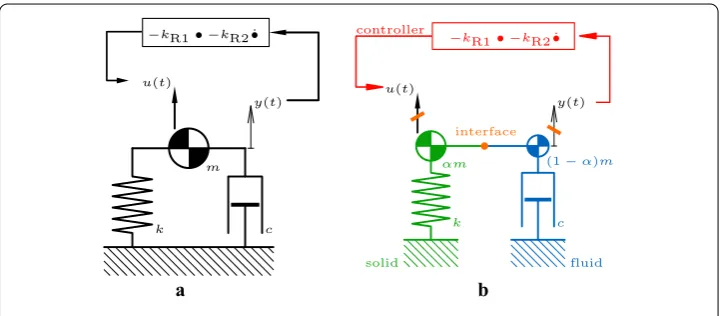
The simplified model problem introduced by [8,9] is extended by a generic control unit. According to [8,9], the system approximating the FSI scenario in the simplest way is the combination of point mass, linear damper and a linear elastic spring. This simplified model problem is illustrated in Fig.1in a monolithic version (a) and a partitioned version (b). The decomposition into three subsystems and the explicit realization of interfaces (each creating an interface constraint equation), is visualized in Fig.1b by the orange separators. Figure 1is described in more detail during the course of this subsection. The features of the newly proposed simplified FSCI model problem can be summarized as follows: the coupling of a first order ordinary differential equation (ODE) representing the fluid flow and a second order ODE representing the structure reproduces the FSI problem. This is extended to the FSCI problem by adding the algebraic ODE of the controller. In the simplified model problem the combination of viscosity/inertia in one subsystem (fluid flow) and stiffness/inertia in the other (structure) also corresponds to the main characteristics of FSI problems. The physics are still dominated by the FSI subproblem, since inertia is limited to the fluid flow and the structure. The controller is only adjusting the dynamics of the structure. An iterative/strong/implicit coupling is applied, meaning all interface constraints are fulfilled strictly using an interface iteration loop. More precisely, we use a Dirichlet/Neumann [10, p. 4517 et seq.] coupling, with a block Gauss–Seidel procedure [11–13]. The monolithic version in sub-figure (a) results in the well-known single degree of freedom (SDoF) system
m¨y(t)+c˙y(t)+ky(t)=u(t), (1)
with its initial conditions y(0)=y0,
˙
y(0)=˙y0.
(2)
Herein the constantsm,c, andkrepresent the mass, the viscous damping and the stiffness. The variables ¨y(t), ˙y(t) andy(t) represent the acceleration, velocity and displacement. The variableu(t) on the right hand side represents the control input. Thus,y0is the initial
displacement and ˙y0is the initial velocity. Equation (1) is equivalent to [8, p. 5], enhanced
by a generic, but representative state-feedback controller. The state-feedback controller equation is defined as
−kR1• −kR2 ˙•
u(t)
controller
y(t)
interface
solid
k c
fluid
αm (1−α)m
−kR1• −kR2 ˙•
u(t)
y(t)
k m
c
a b
u(t)= −kR1y(t)−kR2˙y(t). (3)
The constant factorskR1for the displacement andkR2for the velocity in the control input
are used to tune the controller. Inserting Eq. (3) into (1) one gets
m¨y(t)+(c+kR2) ˙y(t)+(k+kR1)y(t)=0, (4)
with the initial conditions from Eq. (2), which is a controlled SDoF system. In the fol-lowing this is referred to as simplified model problem. This system stays linear and one-dimensional. The reason for this is the treatment of the control inputu(t) as Neumann boundary condition on the SDoF system, which corresponds to a disturbing forcez(t). Therefore no additional displacement degree of freedom is added. This results in pure force control for the considerations in this work.
Monolithic approach
For the temporal discretization of the monolithic model problem the implicit Euler time integrator also called “first order backwards differentiation formula” (BDF1) is used. The BDF1 is defined as:
yn+1=yn+δty˙n+1, ˙
yn+1=y˙n+δty¨n+1. (5)
Hereinδtis the discrete time step size andyn+1andynare the discrete instances of the displacements, velocities ˙yn+1and accelerations ¨yn+1at time stepstn+1 andtn, with n being the time step counter. Rewriting Eq. (5) and applying it to Eq. (4) leads to the time discrete monolithic expression of the coupled system.
m+(c+kR2)δt+(k+kR1)δt2
yn+1−(2m+(c+kR2)δt)yn+myn−1=0 (6)
and its discrete initial conditions y−1=y0−δt˙y0,
y0=y0.
(7)
Thus it is subsequently possible to derive statements, which reflect the choice of the controller parameterskR1andkR2for which the controlled system shows stable dynamics.
Analysis of the time-continuous problem
The stability regioncfor the time-continuous, monolithic simplified model problem Eq.
(4) is derived using its characteristic polynomial. The characteristic polynomial reads p(s)=ms2+(c+kR2)s+(k+kR1). (8)
This is Eq. (4) transformed to the complex s-plane by a Laplace transform, wheresis a complex number. The roots of Eq. (8) are defined as
{s∈C|p(s)=0}. (9)
In this case asymptotically and bounded input bounded output (BIBO) stability coincide [14, p. 63, et seq.] or [15, p. 45, et seq.]. The time-continuous stability regioncresults in
c=
kR1, kR2∈R
max
i=1,2{Re{si}} ≤0
=kR1, kR2∈RkR1≥ −k ∧ kR2≥ −c
. (10)
Hereinsidenote the two poles of the time-continuous problem, which are specified by its
Analysis of the time-discrete problem
In a similar way, the stability regiondfor the time-discrete, monolithic model problem
Eq. (6) is determined. Its characteristic polynomial reads p(z)=m+(c+kR2)δt+(k+kR1)δt2
z2−(2m+(c+kR2)δt)z+m=0. (11)
This is Eq. (6) transformed to the complexz-plane by a matched z-transform. The roots of Eq. (11) are defined as
{z∈C|p(z)=0}. (12)
Finally, the map between the time continuouss-plane and the time discretez-plane is defined as
z=esδt. (13)
The disturbance forcez(t) is not to be mixed up with thezfrom the matchedz-transform. The two basic stability conditions change for the time discrete case [14]. Consequently, the time-discrete regiondformulated in thez-plane results in
d=
kR1, kR2∈R
max
i=1,2{|zi|} ≤1
. (14)
Mapped back to thes-plane with Eq. (13) this reads
d= {kR1, kR2∈R
δ1tln max
i=1,2{|zi|}
≤0} = {kR1, kR2∈RkR1≥ −k
∧ kR2≥ −c−δt(kR1+k)}. (15)
Hereinzidenote the two poles of the time-discrete problem, which are specified by its
eigenvalues.
Clearly recognizable in Eq. (15) is the fact that the time-continuous stability region
crepresenting real physics gets extended to an apparently larger, time-discrete
stabil-ity region d. This has to be taken into account when conducting a simulation based
controller design.
Partitioned approach
The initial step of a partitioned approach is the decomposition of the multi-physics prob-lem into single-physics subprobprob-lems and appropriate interface constraints covering the interactions. This is referred to as partitioning [6] and is shown in Fig.1b.
A preparatory step for reaching a suitable partitioning of the simplified model problem is the reformulation of the ODE Eq. (1) as
(αm)¨y(t)+((1−α)m)¨y(t)+c˙y(t)+ky(t) = u(t)+z(t). (16) The disturbance force on the right hand sidez(t) has to be split up intozF(t) andzS(t),
since Eqs. (17) and (18), which are the partitioned equations, need a disturbance force each. In combination with Eqs. (2) and (3) this leads finally to the partitioned, simplified model problem:
((1−α)m) ¨yF(t)+c˙yF(t)=zF(t), (17)
is referred to as the fluid subsystem (index F),
as the structural subsystem (index S) and
uC(t)= −kR1yC(t)−kR2˙yC(t), (19)
as controller subsystem (index C). The physical interaction is shifted to the interface constraints (index I)
yF(t)−yS(t)=0,
zF(t)+zS(t)=0,
yS(t)−yC(t)=0,
uS(t)−uC(t)=0.
(20)
The initial conditions for the structure are given with yS(0)=y0,
˙
yS(0)=y˙0.
(21)
Thus, the structural domain is represented by the elastic springk and the point mass shareαm, the fluid domain by the linear dampercand the point mass share (1−α)m. The interface constraints cover the interactions between these two domains (FSI) and between structure and controller (SCI).y(t) describes the displacement, which corresponds to the measured output.z(t) is the disturbance (force) originating from the partitioning andu(t) the control input. The interface constraint equations are formulated in Eq. (20).
The parameterα ∈ [0,1) describes the mass distribution between fluid and structural subsystem, i.e.
mS
m =α and mF
m =1−α, (22)
and allows to precisely quantify the added-mass effect [8,10,16], which also applies to FSCI problems. Also other “α”-parameters regarding the dampingcand the stiffnessk would be feasible [8, p. 5]. At this stage only one parameterαassociated with the mass m is considered. In the dominating FSI subproblem the convergence properties of the relaxed iteration factorβAin the limit caseδt → 0 depend only on this one parameter [11, Sect. 3, p. 763].
The temporal discretization of the partitioned simplified model problem Eqs. (17), (18), (19), (20) and (21), with the BDF1 scheme leads to the discrete, partitioned, simplified model problem. It consists of the discrete fluid Eq. (23), structural Eq. (24) and controller subsystem Eq. (25):
zFn+1= (1−α)m+cδt
δt2 y
n+1 F
−(1−αδ)m+cδt t2 y
n
F−
(1−α)m
δt y˙
n F,
zFn+1= GF
ynF+1,
(23)
ynS+1= δt
2
αm+kδt2z n+1
S +
δt2
αm+kδt2u n+1 S
+ αm
αm+kδt2y n
S+
αmδt
αm+kδt2y˙ n S,
ynS+1= GS
znS+1, unS+1,
(24)
unC+1= −kR1δt+kR2
δt y
n+1
C +
kR2 δt y
n C,
unC+1=GC
ynC+1
and the discrete interface equations ynF+1−ynS+1=0, i.e. IFS,y
ynF+1,ynS+1=0, (26)
znF+1+znS+1=0, i.e. IFS,z
zFn+1,znS+1=0, (27)
ynS+1−ynC+1=0, i.e. ISC,y
ynS+1,ynC+1
=0, (28)
unS+1−unC+1=0, i.e. ISC,u
unS+1,unC+1
=0. (29)
The operatorsGandIdescribe the input-output relation for the specific subsystem and the interface constraint for the specific coupling, respectively.
The FSI subproblem, i.e. the coupling between fluid and structure, converges to the solution of Eqs. (23), (24), (26) and (27). The emerging system is the “fluid–structure (FS) subsystem”,GFS
unS+1. Accordingly, the converged solution of the SCI subproblem, i.e. the coupling between structure and controller fulfills Eqs. (24), (25), (28) and (29). This leads to a “structure–controller (SC) subsystem”,GSC(zSn+1).
Alternatives of the Gauss–Seidel pattern for three different physical fields Three different alternatives for the serial Gauss–Seidel pattern for the fluid–structure– control interaction problem are described and applied to the partitioned simplified model problem consisting of Eqs. (23)–(29). The resulting nonlinear interface equation system can be solved in different ways. Since in this contribution we want to concentrate on the algorithmic aspects of the overall problem, the simplest iterative technique applying fixed point iterations Eq. (30), accelerated by relaxation Eq. (31) is used [17, p. 652–659]. Applying a Gauss–Seidel pattern, this implies the subsequent solution of all involved single-physics subsystems in each iteration step.
k+1yn+1
S =1AkynS+1+bn. (30)
k+1yn+1
S =β
1AkynS+1+bn
+(1−β)kynS+1,
k+1yn+1
S =βAkynS+1+βbn, (31)
Herein the indexkindicates the iteration counter for the interface iterations, the indexn the counter for the time integration,βdenotes the user-defined relaxation parameter,1A
andβAdenote the unrelaxed and relaxed iteration factors.
For each of those variants the limits of the unrelaxed1Aand the relaxedβAiteration
factors are derived and the optimal relaxation parameterβ∗is calculated. The algorithms in pseudocode notation for the different alternatives can be found in the appendix.
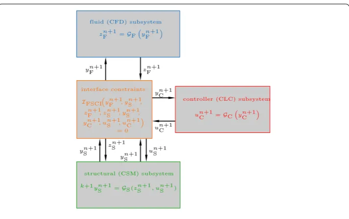
No nesting (FSCI)
IFSCIhas to be solved. In the graphical representation as a block diagram, each of the
physical fields and the interface equations are outlined by one of the blocks. The arrows describe the input and output quantities, which are passed between the blocks. Applying Eq. (30) to the partitioned, simplified model problem the equations of the algorithm condense down to
k+1yn+1 S
(24)
= GS
kzn+1 S ,kunS+1
(27),(29)
= GS
−kzn+1
F ,ku
n+1 C
(23),(25)
= GS
−GF
kyn+1 F
,GC
kyn+1 C
(26),(28)
= GS
−GF
kyn+1 S
,GC
kyn+1 S
, i.e. k+1ynS+1=1AFSCIkynS+1+bn.
(32)
Hereinbnis the part remaining constant during the iteration process. The limit of the iteration factor
lim
δt→0{1AFSCI} = α−1
α , (33)
shows pure dependency on the mass distributionα.
Supplemented by relaxation, the FSCI scheme shown in Eq. (32) is extended to
k+1yn+1
S =βGS
−GF(kynS+1),GC(kynS+1)
+ (1−β)kynS+1, i.e. k+1ynS+1=βAFSCIkynS+1+βbn.
(34)
The limit of the iteration factor
znF+1=GF
ynF+1
yn+1
F znF+1
ynC+1
un+1 C
yn+1
S yn+1 S
zn+1
S un+1 S
k+1yn+1
S =GS(znS+1, unS+1)
un+1 C =GC
yn+1
C interface constraints
IFSCI
yn+1 F , ynS+1, zn+1
F , znS+1, ynS+1, ynC+1, unS+1, unC+1
= 0
fluid (CFD) subsystem
structural (CSM) subsystem
controller (CLC) subsystem
lim δt→0
βAFSCI
= α−β
α , (35)
is now clearly determined by the mass distributionαand the relaxation parameterβ. The optimal relaxation parameter becomes
βFSCI∗ =
αm+kδt2
m+(c+kR2)δt+(k+kR1)δt2
. (36)
Each term in the denominator is positive, non-zero for physically relevant parameters and stable controller settings according to Eq. (10). Thus, it can always be found.
Nesting of the FSI sub–problem ([FS]CI)
The acronym [FS]CI denotes the specific iterative coupling scheme illustrated in Fig.3, where the Gauss–Seidel communication pattern is depicted with nesting of the FSI sub-problem, which is indicated by bracketing [FS]. The nesting of sub-problems corresponds to the inclusion of bi-coupling schemes mentioned in [18]. As it can be seen in Fig.3, two interface constraint equations are to be set up. One for the FS subproblem (inner inter-face constraints)IFSIand one for the overall coupling between the FS subsystem with the
control subsystem (outer interface constraints)I[FS]CI. At first the FS loop is iterated with
constant control input until convergence. The converged values are used as information for the iterations of the outer loop. If the outer loop does not converge, the algorithm has to return to the inner loop. Before proceeding to the next time step, inner and outer loop have to be converged. The scheme is again applied to the partitioned simplified model problem. Since the pure FSI is solved in its own iteration loop, it is possible to calculate the best relaxation factor once for the FSI problem, involving two coupled fields and for the complete FSCI problem involving three coupled fields.
fluid (CFD) subsystem
zn+1
F =GF
yn+1
F
zn+1 F
yn+1 F
inner interface constraints
IFSI
ynF+1, ynS+1, zn+1
F , znS+1
= 0
un+1 C =GC
yn+1
C
yn+1
S znS+1
yn+1
C unC+1
yn+1 S
un+1 S
ynS+1=GS
znS+1, unS+1
outer interface constraints
I[FS]CIyn+1 S , ynC+1, unS+1, unC+1= 0 structural (CSM) subsystem
controller (CLC) subsystem
FSI
The inner FSI fixed-point iteration of the algorithm condenses down to
l+1kynS+1 (24)
= GS
lkznS+1,kunS+1=const.
(27)
= GS
−lkzFn+1,kunS+1=const.
(23)
= GS
−GF
lkynF+1
,kunS+1=const.
(26)
= GS
−GF
lkynS+1
,kunS+1=const.
, i.e. l+1kynS+1=1AFSIlkynS+1+kbn.
(37)
Herein the iteration counterlis used for the inner iteration loop and the iteration counter kfor the outer iteration loop. For the inner FSI fixed point iteration the constant part is
kbn.
The limit of the inner iteration factor lim
δt→0{1AFSI} = α−1
α , (38)
shows pure dependency on the mass distributionα.
Supplemented by relaxation the inner FSI part of the scheme reads
l+1kynS+1=βGS
−GF(lkynS+1),ku n+1 S =const.
+(1−β)lkynS+1,
i.e. l+1kynS+1=βAFSIlkynS+1+βkbn.
(39)
The limit of the inner iteration factor lim
δt→0
βAFSI
= α−αβ, (40)
now is obviously determined by the mass distributionαand the relaxation parameterβ. The optimal relaxation parameter becomes
βFSI∗ =
αm+kδt2
m+cδt+kδt2. (41)
It can always be found since each term in the denominator is positive non-equal to zero for physically relevant parameters independent of the controller settings.
Assuming convergence, the inner FSI fixed-point iteration can be substituted by the equivalent FS subsystemGFS
kun+1 S
for analyzing the outer [FS]CI fixed-point iteration. Consequently, this outer [FS]CI fixed-point iteration of the algorithm condenses down to
k+1yn+1
S =GFS
kun+1 S
(29)
= GFS
kun+1 C
(25)
= GFS
GC
kyn+1 C
(28)
= GFS
GC
kyn+1 S
, i.e. k+1ynS+1=1A[FS]CIkynS+1+bn.
(42)
Herein the factorbnremains constant during all iterations. The limit of the outer iteration
factor lim δt→0
1A[FS]CI
=0, (43)
Supplemented by relaxation the outer [FS]CI part of the scheme reads
k+1yn+1
S =βGFS
GC(kynS+1)
+(1−β)kynS+1, i.e. k+1ynS+1=βA[FS]CIkynS+1+βbn.
(44)
The limit of the outer iteration factor lim
δt→0
βA[FS]CI
=1−β, (45)
shows pure dependency on the relaxation parameterβ. The optimal relaxation parameter becomes
β[FS]CI∗ =
m+cδt+kδt2 m+(c+kR2)δt+(k+kR1)δt2
. (46)
Each summand in the denominator is positive and non-equal to zero for physically relevant parameters and stable controller settings according to Eq. (10). Thus, it can always be found.
Nesting of the SCI sub–problem (F[SC]I)
The acronym F[SC]I denotes the specific iterative coupling scheme illustrated in Fig.4, where the Gauss–Seidel communication pattern is depicted with a nesting of the SCI subproblem, which is made clear by bracketing [SC]. Comparable to the [FS]CI problem, for the F[SC]I problem two interface equations are also to be set up.ISCIfor the inner
andIF[SC]Ifor the outer iteration loop. As already indicated, the solution procedure for
the F[SC]I problem is done just the other way around like in the [FS]CI problem. Accordingly, first the SC loop is iterated applying a constant disturbance force until convergence. The converged values are used as information for the iterations of the outer loop. If the outer loop does not converge, the algorithm has to return to the inner loop. Before proceeding to the next time step, inner and outer loop have to be converged. The scheme is again applied to the partitioned simplified model problem. The inner SCI fixed-point iteration of the algorithm condenses down to
fluid (CFD) subsystem
zn+1 F =GF
yn+1
F
zn+1 F yn+1
F
outer interface constraints
IF[SC]Iyn+1
F , ynS+1,
zn+1
F , znS+1
= 0
un+1 C =GC
yn+1 C
yn+1 S zn+1
S
yn+1
C unC+1
yn+1
S unS+1
yn+1 S =GS
zn+1 S , unS+1
inner interface constraints
ISCI
yn+1
S , ynC+1,
un+1
S , unC+1
= 0
controller (CLC) subsystem
structural (CSM) subsystem
SCI
l+1kynS+1 (24)
= GS
kzn+1
S =const.,lkunS+1
(29)
= GS
kzn+1
S =const.,lkunC+1
(25)
= GS
kzn+1
S =const.,GC
lkynC+1
(28)
= GS
kzn+1
S =const.,GC
lkynS+1
, i.e. l+1kynS+1= 1ASCIlkynS+1+kbn.
(47)
Again the iteration counterlis used for the inner iteration loop and the iteration counter kfor the outer iteration loop. As defined for the FSCI and the [FS]CI problem,kbnis the constant part of the inner iteration loop.
The limit of the inner iteration factor lim
δt→0{1ASCI} =0, (48)
is always zero independently of the parameter setting.
Supplemented by relaxation the inner SCI part of the scheme reads
l+1kynS+1=βGS
kzn+1
S =const.,GC(lkynS+1)
+(1−β)lkynS+1,
i.e. l+1kynS+1=βASCIlkynS+1+βkbn.
(49)
The limit of the inner iteration factor lim
δt→0
βASCI
=1−β, (50)
shows pure dependency on the relaxation parameterβ. The optimal relaxation parameter becomes
βSCI∗ =
αm+kδt2
αm+kR2δt+(k+kR1)δt2
. (51)
αmand (k+kR1)δt2in the denominator are positive and non-equal to zero for physically
relevant parameters and stable controller settings according to Eq. (10).
Thus, the optimal relaxation factor can always be found by additionally requiring kR2δt= −αm+(k+kR1)δt2.
Assuming convergence, the inner SCI fixed-point iteration can accordingly be substi-tuted by the equivalent SC subsystemGSC
kzn+1 S
for analyzing the outer F[SC]I fixed-point iteration. Consequently, this outer F[SC]I fixed-fixed-point iteration of the algorithm condenses down to
k+1yn+1
S =GSC
kzn+1 S
(27)
= GSC
−kzn+1
F
(23)
= GSC
−GS
kyn+1 F
(26)
= GSC
−GF
kyn+1 S
, i.e. k+1ynS+1=1AF[SC]IkynS+1+bn.
(52)
The limit of the outer iteration factor lim
δt→0
1AF[SC]I
= α−1
α , (53)
Supplemented by relaxation the outer F[SC]I part of the scheme reads
k+1yn+1
S =βGSC
−GF
kyn+1 S
+(1−β)kynS+1,
i.e. k+1ynS+1=βAF[SC]IkynS+1+βbn.
(54)
And the limit of the outer iteration factor lim
δt→0
βAF[SC]I
= α−β
α , (55)
now is obviously determined by the mass distributionαand the relaxation parameterβ. The optimal relaxation parameter becomes
βF[SC]I∗ =
αm+kR2δt+(k+kR1)δt2
m+(c+kR2)δt+(k+kR1)δt2
. (56)
It always exists since the denominator is positive and non-equal to zero for physically relevant parameters and stable controller settings according to Eq. (10).
From the simplified model problem it can be concluded that all three types of the Gauss– Seidel schemes show unconditional stability for reasonable physical parameters and stable controller settings. Furthermore, it was possible to derive optimal relaxation parameters
β∗. Thus, the schemes can be subsequently applied to a multi-degree of freedom problem for further investigations, which have not been possible with the simplified model problem.
Numerical results for a multi-degree of freedom FSCI problem
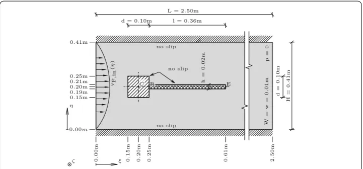
The inspiration for the multi-degree of freedom FSCI experiment were the numerical benchmarks proposed in [19,20, p. 195–197]. Since the investigations should go beyond the study of the pure FSI effects, the experimental setup had to be slightly modified. All in all, the principle arrangement remains the same and can be seen in Fig.5.
In contrast to the rigid cylinder in [19], a square, as suggested in [20], is placed in the channel. To this rigid square an elastic flag (charactersRtoE) is attached. The square and flag are placed asymmetric in the channel in order to stimulate a fast onset of the excitation mechanism depicted in Fig.7. The phenomenology of the problem is described in [19,20].
In the following we are actively trying to influence the dynamics of the structure by a controller, extending the FSI to the FSCI problem. The main objective of this is to reduce
0.41m
0.25m 0.21m 0.20m 0.19m 0.15m
0.00m
0
.
00m
0
.
15m
0
.
20m
0
.
25m
0
.
61m
2
.
50m
H=0
.
41m
d=0
.
10m
h=0
.
02m
d = 0.10m
L = 2.50m
l = 0.36m
ζ
E
W=w=0
.
01m
ξ η
C R no slip
no slip no slip
p=0
vF
,
in
(
η
)
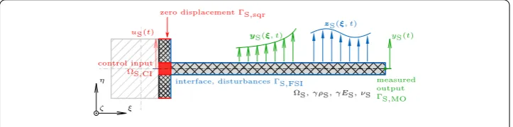
Fig. 6 Computational structural mechanics high fidelity model
or in the best case entirely suppress the amplitude of the end-point displacement at point E. Similar to the simplified model problem, the control input is a Neumann boundary condition, which is applied at the root point of the flagR. For the design of the controller, a reduced order model is necessary [15,21], which is exemplarily shown in Fig.8. This low fidelity structural model was only used for the controller. In the coupled FSCI simulation the structure was simulated like in classical FSI by the high fidelity model depicted in Fig.6.
For all simulations of the multi-degree of freedom FSCI problem the open-source soft-ware Kratos Multi-Physics [22,23] was used.
Description of the subsystems involved
Just as mentioned in the introduction, the FSCI problem involves three subsystems, namely a fluid flow, a structural mechanics part and a controller.
At first the computational fluid dynamics (CFD) subsystem is introduced. The main dimensions and the boundary conditions of the problem can be seen in Fig.5. The time constant inlet velocity is described by the function
vF,in(η)=vmax4η
H
1− η H
. (57)
This is a quadratic parabola withvmaxat its peak value. Hereinηis the coordinate running
form the bottom of the channel to its widthH. The material parameters for the fluid flow are chosen in accordance to the CFD3 specifications in [19], leading to a strongly unsteady flow with vortex shedding. This vortex shedding is additionally supported by the aforementioned eccentric placement of the square in the channel. Thus the following specifications are chosen:ρF = 1000 kg/m3, νF = 0.001 m2/s andvin = 2 m/s, which
leads to a Reynolds number Re = 200. The fluid flow is discretized by a monolithic finite element formulation with triangular elements developed in [24], using a variational multi-scale (VMS) method for stabilization. In this case, the integration in time is done by a second order backwards differentiation formula (BDF2). The BDF2 scheme approximates the velocity as
˙
yn+1= 1
δt 3 2y
n+1−2yn+ 1
2y
n−1
. (58)
Next, the computational structural mechanics subsystem (CSM) is presented. The CSM subsystem is represented by a high fidelity multi-degree of freedom model which is the initially suggested CSM system as proposed in [19]. The specifications of the high fidelity model can be seen in Fig.6.
Herein,zs(ξ, t) is the disturbance force from the fluid flow andyS(ξ, t) is the displacement
of the structure at the interface. Again one can see that the control inputuS(t) is applied
only at the root point of the elastic flag and the displacementyS(t) is measured solely at
its tip. The special aspect of the high fidelity model is the back part of the square (finely crosshatched), which is originally assumed to be rigid in [19], but is considered elastic in the current investigation. It is used to linearly distribute the root point excitation along the back side of the square in order to match the ALE boundary conditions of the fluid domain. Therefore a pseudo material withν = 0 andρ = 0 is set, to avoid artificially introduced deformations and inertia effects at the back of the square. The high fidelity CSM model itself is discretized by a structured mesh of 4-node (2D) non-linear, fully integrated plane stress elements formulated in Total Lagrangian kinematics. In this case the temporal discretization is performed by Newmark’s method. The material used for the simulations is a linear St. Venant Kirchhoff material with the parametersρs=1000 kg/m3, ES=5.6·106N/m2andνS=0.4. The values used for the simulations match the CSM2
benchmark of [19] scaled by the factor ofγ. The gravity constant is set tog =2 m/s2and
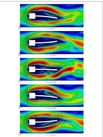
is acting inξdirection. Figure7shows an extract of the simulation results for one second by using the parameters for fluid flow and structural model described in this subsection (γ =102) in order to show the deformation mechanism. The figure shows the deformed mesh and the velocity contours. The controller is not activated yet. The displacements at pointEwith and without activated controller are plotted in Figs.10and11.
The meshes on the interface of fluid and structure subsystem coincide, thus no additional mapping operation is necessary.
The third subsystem consists of a low fidelity CSM model, which is implemented in the controller and the control law itself. In the low fidelity CSM model the overall structural dynamics are condensed to a single degree of freedom system. The low fidelity model can be seen in Fig.8. It has been derived from the high fidelity multi-degree of freedom model. The structural model itself is approximated by a simple second-order ODE, which matches the boundary conditions of the high fidelity model and is used by the controller to calculate uS(t). The distributed displacements yS(ξ, t) between pointsR and E are
approximated by quadratic shape functions, which should be a good enough assumption for the dominant mode shape of the investigated problem (see Fig.7). They are defined asyu(ξ) = 1−
ξ−ξR/l
2
for the control inputuS(t) andyx(ξ)=
ξ−ξR/l
2
for the state variablexS(t). Thus, the real physics of the high fidelity model reduces to
(γm)¨xS(t)+(γk)xS(t)=(γb0)uS(t)+zS(t). (59)
In the latter equation the single statexS(t) directly corresponds to the measured output
yS(t) at the end pointEresulting inyS(t)=xS(t). The parameterb0, which is associated
with the control input at the root pointR,uS(t), is used to replace the root point excitation,
Fig. 7 Deformed structure with velocity contours and deformed finite element mesh for the numerical experiment from 10.0 to 11.0 s by snapshots in steps of 0.25 s
interface
ζ ξ
η
uS(t)
zS(ξ, t)
yS(ξ, t)
0
0
m γc,γk
xS(t)
control input
zS(t)
meas. output =yS(t)
γb0
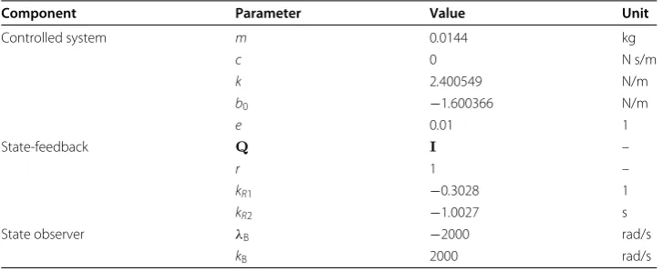
Table 1 Values selected for controller parameters
Component Parameter Value Unit
Controlled system m 0.0144 kg
c 0 N s/m
k 2.400549 N/m
b0 −1.600366 N/m
e 0.01 1
State-feedback Q I –
r 1 –
kR1 −0.3028 1
kR2 −1.0027 s
State observer λB −2000 rad/s
kB 2000 rad/s
work (PvW) with a distributed cross sectional massμ=ρwh, wherewis the width,hthe height of the cross section and withEI is the distributed sectional stiffness, leads to
μ
ξR+l
ξR
y2x(ξ)dξx¨S(t)+EI
ξR+l
ξR
y2x(ξ)dξxS(t)
=μ
ξR+l
ξR
yx(ξ)yu(ξ)dξu¨S(t)
+EI ξR+l
ξR
yx(ξ)yu(ξ)dξuS(t)+
i
yx(ξi)zηS(ξi, t).
(60)
The last term of Eq. (60) denotes the discrete disturbance forces coming from the nodes ion the interface mesh of the fluid domain which are to be summed up here. The open parameters in Eq. (59) can be obtained as:
m= μl 5 =
ρwhl 5 ,k=EI
l 5 =
ESwh3
4l3 ,
b0= −EI
2l 15 =
ESwh3
6l3 ,zS(t)=
i
ξi−ξR l
2
zηS(ξi, t).
(61)
Those approximations are applied to the centerline of the structure and have to be pro-jected to the surfaces of the flag by appropriate projection operations. The time discrete low fidelity CSM model is finally given with the adapted time discretization Eq. (24) from the simplified model problem. The equivalent values to match the multi-degree of free-dom model form,kandb0can be found in Table1. Those parameters can be scaled by
the parameterγ accordingly.
With the low fidelity CSM model, the controller can be designed. In this case, a state-feedback control following state observer is implemented, which is state of the art for modern methods for controller design and is also used in the context of many applications in control theory. Herein, the controller state feedback matrix is specified via a linear-quadratic regulator approach (LQR) and the observer output-feedback matrix is set via pole placement as generally described in [15,21]. The block diagram can be seen in Fig.9. The controlled system, which is seen by the controller, is represented by the equation
(γm)¨y(t)+(γc)˙y(t)+(γk)y(t)=(γb0)u(t)+ez(t), (62)
KR
y0, ˙y0 z
x20
yd = 0 u y
x −
controlledsystem (γm) ¨y+ (γc) ˙y+ (γk)y=
(γb0)u+ez
reduced stateobserver
open- and closed-loopcontroller
Fig. 9 Block diagram for the controlled system with following state observer [21], p. 334
forcez(t) is applied from recorded FSI simulations of the system. The system is rewritten in state-space representation, withx1:=y(t) andx2:=y(t) being the entries in the state˙
vectorx=[x1, x2]T, reading
˙ x1
˙ x2
=
0 1 −k
m − c m
x1
x2
+
0
b0 m
u(t)+
0
e m
z(t),
i.e. x˙=Ax+Bu(t)+Ez(t)
(63)
and the output equation
y(t)=
1 0 x1 x2
,
i.e. y(t)=Cx.
(64)
where A, B,C andE are constant matrices. Since the system is fully controllable and fully observable, state-feedback control and state observer are possible. Thus a control law similar to the one presented for the model problem can be used. This is given by
u(t)= −KRx, (65)
withKR=[kR1kR2] being the constant state feedback matrix. Herein the constants inKR
are determined with the LQR approach described in detail in [21, chapter 7]. This involves user-definable weightsQ∈R2,2related to state thexandr∈R1,1for control inputu(t). With an appropriate choice ofQ=Q(γ) andr=r(γ) the state-feedback matrix becomes independent ofγ, because alsoA=A(γ),B=B(γ) andC=C(γ).
Since the displacementy(t), being state one, should be measured during the simulations, it is directly accessible (x1=y(t)). The second state should not be measured directly and
thus needs an approximation. This approximationx2 ≈x2is done from measurements
˙
x=Ax+Bu,
i.e.
˙ y(t)
˙ x2
=
0 1 −k
m − c m
y(t) x2
+
0
b0 m
u(t). (66)
Conducting the observer design and applying the BDF2 scheme results in xn1+1=yn+1,
[LHS]xn2+1= −1
δt
−2x2n+1 2x
n−1 2
+[RHS]yn+1, xn2+1=x2n+1+kByn+1,
un+1= −kR1x1n+1−kR2xn2+1,
(67)
where
[LHS]= 3
2δt −aB+bBkR2= 3 2δt +
c
m+kB+ b0
mkR2, [RHS]=eB−bB(kR1+kR2kB) ,
= −c m+kB
kB−
k m−
b0
m(kR1+kR2kB) (68)
and ˜x2results from the design of the reduced state observer.
For multi-degree of freedom problems, like the one presented in this section, it is not possible to derive an optimal relaxation parameterβ∗ [11, p. 769] as was done for the simplified model problem. Thus in this paper it is computed by Aitken acceleration as proposed for FSI problems in [8,11].
Residual calculation and numerical accuracy
The overall coupled partitioned FSCI problem as well as the fluid subsystem were solved by an iterative approach. For the structural and the controller subsystem a direct solver was used. For iterative solution procedures the residual calculation and the accuracy of the solution play an important role in order to gain correct results [2,27, p. 201]. In the following a closer look is taken to the iterative solution of the interface equation system. For FSI [28] shows that in order to achieve the desired accuracy for the coupled problem using an iterative approach, the numerical accuracy of the solution of the subsystems has to be at least two orders of magnitude higher than the desired numerical accuracy of the coupled system. Thus, it makes sense to use the outcome of those investigations also for the FSCI problem.
Another crucial part is the calculation of the residual of the interface equation system. Since we are dealing with Dirichlet–Neumann coupling, it is obvious to calculate the residual vectorRy from the interface displacements, which correspond to the structural displacementsySof the high fidelity model. This means
kRy =ky
S−k−1yS. (69)
The convergence at the interface is achieved if
kR
yndof ≤εI. (70)
where||. . .||denotes theL2norm of the residual vector andεIis the desired accuracy on the interface. The indexkdenotes the iteration counter. The residual is normalized by the square root of the number of degrees of freedom on the interfacendof [28]. For the results
Table 2 Recommendation for the numerical accuracy of solvers and interface iterations on basis of [28]
FSI FSCI [FS]CI F[SC]I
εF 10−(p+2) 10−(p+2) 10−(p+4) 10−(p+4)
εS 10−(p+2) 10−(p+2) 10−(p+4) 10−(p+4)
εinner
I 10−p 10−p 10−(p+2) 10−(p+2)
εouter
I – – 10−p 10−p
0.0·10+0 2.0·10−2 4.0·10−2 6.0·10−2
−2.0·10−2
−4.0·10−2
−6.0·10−2
measured
output
y
in
[m]
0 2 4 6 8 10 12 14
time t in [s]
14.5 15 14
FSI FSCI with LQR
Fig. 10 Results: FSI and FSCI with LQR (γ=102)
table, the proportions of values for the stopping criteria of the coupled simulations for the different variants of partitioned simulation patterns are listed. At first the overall desired numerical accuracy, which finally is to be achieved for the overall coupled simulation, was selected in this case to bep=7, resulting in a value ofεI = 10−7for the interface iterations. Afterwards the values ofεFfor the fluid solver andεSfor the structural solver as well as for the inner interface iteration loopεIinnerand the outer interface iteration loop
εouter
I were adopted according to the criteria described above.
Presentation and interpretation of the results
The simulations were conducted for 15 s and the measured output, i.e. the tip displacement (pointE) of the elastic flag, has been plotted. The result for a pure FSI and a FSCI simulation with no nesting for a scaling factorγ =102andγ =104can be seen in Figs.10and12.
Additionally the results for the controlled system can be seen in an amplified version for
γ =102in Fig.11. One can see that the controller applied to the root pointRof the flag is able to reduce the magnitude of the tip displacement at pointEin the order of magnitude of almost 102. In Figs.10,11,12and13the horizontal axis represents evolution in time and is subdivided into divisions of two seconds for the time interval form 0 to 14 s and is stretched for the time interval from 14 to 15 s. The vertical axis represents the measured output corresponding to the tip displacement of the flag. The vertical axes in Figs.10and
11have a different scaling, but both figures show the same results for FSCI with LQR. Furthermore, the remaining oscillation in Fig.11is more regular than the one measured from the pure FSI simulation.
0.0·10+0 8.0·10−4 1.6·10−3 2.4·10−3
−8.0·10−4
−1.6·10−3
−2.4·10−3
measured
output
y
in
[m] 3.2·10−3
0 2 4 6 8 10 12 14 14 14.5 15 time t in [s]
FSCI with LQR
Fig. 11 Zoomed view: FSCI with LQR (γ=102)
0 2 4 6 8 10 12 14 14 14.5 15 time t in [s]
0.0·10+0 3.0·10−5 6.0·10−5 9.0·10−5
−3.0·10−5
−6.0·10−5
−9.0·10−5
measured
output
y
in
[m]
1.2·10−4
−1.2·10−4
FSI FSCI with LQR
Fig. 12 Results: FSI and FSCI with LQR (γ=104)
more into play and the system becomes softer. This means the eigenfrequencies of the fluid flow start to dominate the system behavior and the nonlinear behavior of the coupled system becomes stronger. It follows that a new controller design has to be conducted. For a value ofγ ≤10−2the structure is too soft and light to be able to control its behavior by a force applied at its rootpointR. The results for such an example can be seen in Fig.13.
In Fig. 14 the overall number of interface iterations per time step for the different schemes applied to the numerical test example are plotted for the factorγ =102for the
0.0·10+0 1.0·10−2 2.0·10−2 3.0·10−2
−1.0·10−2
−2.0·10−2
−3.0·10−2
measured
output
y
in
[m]
0 2 4 6 8 10 12 14
time t in [s]
14.5 15 14
FSI FSCI with LQR
Fig. 13 Results: FSI and FSCI with LQR (γ=10−3)
[FS]CI F[SC]I FSI FSCI
0 3 6 9 12
0 2 4 6 8 10 12 14 14.5 15
total
n
u
m
b
er
of
iterations
time t in [s]
14
Fig. 14 Total number of iterations per time step (γ =102)
Conclusion and outlook
Within this paper, the algorithmic treatment and solution approaches of fluid–structure– control interaction (FSCI) with iterative Gauss–Seidel schemes is discussed. The aim was to conduct a fully coupled co-simulation of the FSCI problem, with the controller actively influencing the dynamics of the system.
The simplified model problem utilized in a first step is representative of the convergence behavior and stability for structural force control. Thus, all three developed variants of the Gauss–Seidel scheme prove unconditional stability for the simplified model problem in case of physically relevant parameters and stable controller settings. Furthermore, an optimal relaxation factorβ∗could be determined for the simplified model problem. Hence, the simplified model problem is qualitatively capable of constituting the basic properties of the FSCI problem concerning stability and convergence. For the non-linear multi-degree of freedom problem this means one can conclude from the simplified model problem that it should be possible to reduce the displacement significantly by applying a controller with an appropriate set of controller parameters. Since Aitken acceleration is utilized instead of a constant relaxation factor, the schemes developed are supposed to converge in the multi-degree of freedom case. However, since the simplified model problem only covers the main effects of the FSCI problem (e.g. the added mass effect), no detailed and quantitative conclusions concerning convergence patterns and stability issues can be drawn for the multi-degree of freedom problem.
differ-ent material parameter settings of the CSM subsystem also have shown the limits of the chosen controller type and design. Furthermore they show the limits for controllability of this kind of system by applying a force at the root point of the flag. Investigating the total number of iterations per time step illustrates, that the FSCI scheme with no nesting is the best variant for controlling the selected multi-degree of freedom problem presented in this contribution.
As an outlook, more advanced control laws could be applied to the multi-degree of freedom problem in order to reduce the oscillation even more. Furthermore, the number of iterations could be reduced by using more sophisticated coupling schemes like for example presented in [4,29,30].
Abbreviations
FSI: fluid–structure interaction; FSCI: fluid–structure–control interaction; ODE: ordinary differential equation; SDoF: single degree of freedom system; BDFN: backwards differentiation formula of order N; BIBO: bounded input bounded output; SCI: structure–control interaction; VMS: variational multi-scale; ALE: arbitrary Lagrangian Eulerian; CFD: computational fluid dynamics; CSM: computational structural mechanics; PvW: principle of virtual work; LQR: linear quadratic regulator .
Authors’ contributions
AW, CL, K-UB and RW have prepared the manuscript. All authors read and approved the final manuscript.
Author details
1Chair of Structural Analysis, Technical University of Munich, Arcisstraße 21, 80333 Munich, Germany,2Chair of Automatic
Control Technical University of Munich, Boltzmannstr. 15, 85748 Garching/Munich, Germany.
Acknowledgements
Not applicable.
Competing interests
The authors declare that they have no competing interests.
Availability of data and materials
The software used is [23].
Consent for publication
Non-exclusive rights of use.
Ethics approval and consent to participate
Not applicable.
Funding
Not applicable.
Appendix
Algorithm 1:Pseudocode for the partitioned FSCI scheme (no nesting).
// initialize states, i.e. set ICs… kendx0
F←−xinitF ;kendx0S←−xinitS ;kendx0C←−xinitC
// initialize displacements and measured output… kendy0
S←−yinitS ;kendyS0←−yinitS // time loop…
forn←−0to n←−nend−1do
// predict displacements and measured output… 0yn+1
S ←−kendynS;0y n+1
S ←−kendynS
// interface iteration loop, i.e. FSCI loop…
fork←−0to k←−kmaxdo
// map displacements from solid to fluid…
// and copy measured output from solid to controller…
kyn+1
F ←−My
kyn+1
S
ky
Cn+1←−kySn+1
// solve fluid and controller in parallel…
kzn+1
F ←−G
kxn+1
F
F
kyn+1 F
kun+1
C ←−G
kxn+1
C
C
kyn+1 C
// map forces from fluid to solid…
// and copy control input from controller to solid…
kzn+1
S ←−Mz
kzn+1
F
kun+1 S ←−ku
n+1 C // solve solid… k
yn+1 S kyn+1
S
←−G
kxn+1 S
S
kzn+1 S ,kunS+1
// calculate residuum of displacements and measured output… kRn+1
y ←−kynS+1−k−1y n+1 S kRn+1
y ←−kynS+1−k−1ynS+1 kRn+1
y,y :=
kRn+1 y kRny+1
// check for convergence …
kεn+1←−kRn+1 y,y /√ndof
ifkεn+1<maxεthen break
end
// update Aitken factor
ifk=0then
0βn+1←−initβ
else
kβn+1←−k−1βn+1k−1Rny,y+1 Tk−1
Rn+1 y,y−kRny,y+1
k−1Rn+1 y,y−kRny,y+1
2
end
// update displacements and measured output… k+1yn+1
S ←−kynS+1+kβn+1kRny+1 k+1yn+1
S ←−kynS+1+kβn+1kRny+1
Algorithm 2:Pseudocode for the partitioned [FS]CI scheme (nesting of [FS] subsystem).
// initialize states, i.e. set ICs… kend
mendx0F←−xinitF ; kend
mendx0S←−xinitS ;kendx0C←−xinitC
// initialize displacements and measured output… kend
mendy0S←−yinitS ; kend
mendy0S←−yinitS // time loop…
forn←−0to n←−nend−1
// predict displacements and measured output… 0
mendy n+1
S ←−
kend mendy
n S;mend0y
n+1
S ←−
kend mendy
n S
// outer interface iteration loop, i.e. [FS]CI loop…
fork←−0to k←−kmax
// copy measured output from solid to controller… kyn+1
C ←−mendky n+1 S
// solve controller…
kun+1
C ←−G
kxn+1
C
C
kyn+1 C
// copy control input from controller to solid… kun+1
S ←−kunC+1
// predict displacements… k
0ynS+1←−mendky n+1 S
// inner interface iteration loop, i.e. FSI loop…
form←−0to m←−mmax
// map displacements from solid to fluid… k
mynF+1←−My
k mynS+1
// solve fluid…
k
mznF+1←−G
k mxnF+1
F
k mynF+1
// map forces from fluid to solid… k
mznS+1←−Mz
k mznF+1
// solve solid… k
mynS+1 k mynS+1
←−G
k mxnS+1
S
k
mznS+1,kunS+1
// calculate residuum of displacements… k
mRny+1←−mkySn+1−m−k1ynS+1
// check for inner convergence… k
mεn+1←−mkRny+1/√ndof
if k
mεn+1<maxεthen break
end
// update inner Aitken factor…
ifm=0then
k
0βn+1←−initβ
else
ifdimmkRny+1
=1then
k
mβn+1←−m−k1βn+1 k m−1Rny+1 k
m−1Rny+1−mkRny+1
Pseudocode for the partitioned [FS]CI scheme.(continued).
k
mβn+1←−m−k1βn+1 k m−1Rny+1T
k
m−1Rny+1−mkRny+1
k
m−1Rny+1−mkRny+1 2
// update displacements… k
m+1ynS+1←−mkySn+1+mkβn+1mkRny+1
end
// calculate residuum of measured output… kRn+1
y ←−mendkyS
n+1− k−1 mendyS
n+1
// check for outer convergence…
kεn+1←−kRn+1 y /√ndof
ifkεn+1<maxεthen break
end
// update outer Aitken factor…
ifk=0then
0βn+1←−initβ
else
kβn+1←−k−1βn+1 k−1Rny+1 k−1Rn+1
y −kRny+1
end
// update displacements and measured output… k+1
mendy n+1
S ←−mendky n+1 S k+1
mendyS
n+1←− k
mendyS
n+1+kβn+1kRn+1 y
![Fig. 3 Block diagram for [FS]CI scheme](https://thumb-us.123doks.com/thumbv2/123dok_us/9579207.1940757/9.595.117.478.494.710/fig-block-diagram-for-fs-ci-scheme.webp)
![Fig. 4 Block diagram for F[SC]I scheme](https://thumb-us.123doks.com/thumbv2/123dok_us/9579207.1940757/11.595.119.479.503.710/fig-block-diagram-for-f-sc-i-scheme.webp)
![Fig. 9 Block diagram for the controlled system with following state observer [21], p. 334](https://thumb-us.123doks.com/thumbv2/123dok_us/9579207.1940757/18.595.120.477.85.284/fig-block-diagram-controlled-following-state-observer-p.webp)
![Table 2 Recommendation for the numerical accuracy of solvers and interface iterationson basis of [28]](https://thumb-us.123doks.com/thumbv2/123dok_us/9579207.1940757/20.595.115.480.110.318/table-recommendation-numerical-accuracy-solvers-interface-iterationson-basis.webp)
