Supplementing Stochastic Stability
∗
Philip R. Neary
†August 29, 2013
Abstract
This paper uses a game where actions are strategic complements, the “Language
Game” of Neary (2012), to highlight three often-overlooked properties that can affect the set of stochastically stable equilibria when agents are myopic best-responders. They are, (i) the revision protocol (who is afforded an opportunity
to act and when), (ii) how players make mistakes (logit vs uniform), and (iii) network architecture (who is connected to whom). The canonical homogeneous
agent model is robust to each of these properties, but care should be taken when invoking stochastic stability in more complex models, in particular those with
heterogeneous agents. Lastly, the paper uses the measure of group’s
connected-ness from Young (2001), how closely knit it is, and shows that a group must be arranged in this way if it wants to preserve its preferred action (e.g. preserve a spoken language) in the long run.
∗Thanks to Prashant Bharadwaj, Vince Crawford, Colette Ding, Francesco Feri, Chris Gee,
Chuly-oung Kim, WooyChuly-oung Lim, Melanie Luhrmann, Juan Pablo Rud, and especially Sarada, Matt Jackson, and Joel Sobel for all their help.
†Email: [email protected]; Web: https://sites.google.com/site/prneary/. Address:
1
Introduction
Perhaps the simplest large population coordination problem is one where a large group of homogeneous players reside on a fully connected network, and interact pairwise via a common 2×2 game of pure coordination. Famously, Kandori, Mailath, and Rob(1993) (hereafter KMR) and Young(1993) showed that if this setting is played repeatedly by short-sighted optimising agents who are prone to the occasional mistake, then uniform adoption of the locally risk-dominant action is the most likely, so-called stochastically stable equilibrium. Peski (2010) extended this equilibrium selection result to arbitrary networks, showing that uniform adoption of the locally risk-dominant action is always a stochastically stable equilibrium, and uniquely so if the network satisfies a mild density condition.1
While this result put stochastic stability on the map as an equilibrium selection device, it suffered from much criticism. Bergin and Lipman(1996) pointed out that the set of stochastically stable equilibria is not robust to the manner in which players make mistakes. In particular, they showed that any strict equilibrium of the stage game can be rendered stochastically stable for a suitably chosen model of mistakes. However, despite this critique, researchers continue to invoke stochastic stability, typically assuming one of two parameterisations of mistakes: (i) the uniform mistakes of KMR and Young
(1993), where the likelihood of a mistake is independent of everything - the history, the current state, etc., and (ii) the payoff-dependent, “logit”, mistakes introduced first in
Blume (1993).2
In this paper, I use the Language Game of Neary (2012) to highlight three other properties that can affect the selection made by stochastic stability. These properties are often overlooked. While such oversight does not raise concern for the homogeneous agent models listed above, they can matter once any complexity is introduced into the game form. Given the abundance of heterogeneous games that are studied, and the benefits reaped from applying stochastic stability in such games, perhaps more care
1Variants of this result existed already for some particular network structures:Ellison(1993)Ellison
(2000), andBlume(1993) showed risk dominance was uniquely stochastically stable when players are arranged on a circle, torus, and lattice respectively. Jackson and Watts (2002) show that uniform adoption of either action is stochastically stable when players are arranged in a star - the star network being an example of a network that fails Peski’s density condition.
2The result ofPeski(2010), is robust to a wide class of mistake models that includes both of the
should be taken. In particular, I will show that when some properties are held fixed, there can be discontinuities in the selection correspondence (formally, failures of lower hemicontinuity). The Language Game is ideal as a vehicle to identify these issues since it is the simplest possible extension of the canonical model - effectively just doubling it so as to allow heterogeneity in preferences.
To illustrate how these issues matter, it makes sense to be precise about the prop-erties alluded to above. This entails carefully spelling out how stochastic stability is applied. The underlying primitive is always a large population game with more than one equilibrium (hence the selection conundrum). This setting gets repeated with inter-est being in where behaviour, modelled as population dynamics, will lead to. Dynamics have four components. First, there is the revision protocol; this specifies how it is decided which players will be afforded a chance to change their action in a given pe-riod. Second, it is assumed that individual players follow some simple updating rule, a
heuristic, when afforded a revision opportunity. By far and away the most commonly invoked rule, and the one that I focus on in this paper, is myopic best-response to the previous period’s population profile.3 Third, it is assumed that players occasionally
de-viate from the heuristic, by choosing an action not prescribed by it; this is interpreted in economics as players making mistakes, and as mutations in biology. Lastly, time goes forever so that long run effects have time to “kick in”.
There are three revision protocols that pervade the literature. The first of these is asynchronous learning (Binmore and Samuelson, 1997; Benaim and Weibull, 2003;
Blume,1993,2003). The assumption here is that each period one, and only one, player is afforded a revision opportunity, and that all players have positive probability (often assumed to be equal across agents) of being this individual. The second is known as
independent inertia (Samuelson, 1994; Kandori and Rob, 1995), where every period, each agent has a strictly positive probability (again, typically assumed equal across agents) of not being afforded a revision opportunity. The last is the best reply-dynamic, that affords every player a revision opportunity each period with probability one.4
3One rule that has received much attention is imitation, whereby a player mimics the behaviour of
someone whose current payoffoutperforms his own. In this case, the requirement on a game having multiple equilibia is not essential its study to be interesting - seeEshel, Samuelson, and Shaked(1998) for a situation where the local interaction is a prisoner’s dilemma-esque exchange, and imitation can lead to “coordination” on the Pareto-efficient, albeit strictly dominated, action.
4The best-reply dynamic can be thought of as independent inertia with zero inertia. This allows
Coupling a revision protocol with a behavioural rule (in this case, myopic best-response) defines adeterministic population dynamic(an “adjustment process”); further assuming that players will occasionally deviate from this rule (make a mistake) generates anoisy population dynamic (a “stochastic adjustment process”). Uniform mistakes can be matched with each of the revision protocols listed above. Logit mistakes, however, are typically only paired with asynchronous learning.5 Thus, I consider a total of four
(= 3 × 1 + 1) possible noisy population dynamics, and so in theory, four different predictions. However, it will be shown that the noisy dynamic based on asynchronous learning with uniform mistakes generates the same prediction as that of a dynamic based on independent inertia with uniform mistakes, and so the total number of noisy dynamics is further reduced to three. Each dynamic is composed of a deterministic
component and anoise component. They are,
D1 : best-reply +uniform mistakes
D2 : asynchronous learning / independent inertia +uniform mistakes
D3 : asynchronous learning +logit mistakes
I am not advocating any one of these dynamics over another. Rather I am just pointing out that if equilibrium selection is the goal, then the choice can matter. As such, perhaps some justification should be given when a particular dynamic is used (as is the case when invoking a particular equilibrium refinement). For example, there are quite possibly situations in which a particular revision protocol is more appropriate than another - asynchronous learning is probably a better choice if agents can respond at any moment like in a continuous time setting; Experimental work may hold the key in determining precisely how agents deviate from basic rules of thumb, and this might lend credibility for a particular model of mistakes; etc.
The last property that I focus on is not a component of the dynamics, but rather of the stage game. As mentioned before, Peski (2010) shows that risk dominance is selected in the canonical, homogeneous agent model, and this selection result is robust for all of the noisy dynamics listed above and for any network structure. However,
5Al´os-Ferrer and Netzer (2010) examine how robust the prediction with logit mistakes is to the
the homogeneous setting is special and for some purposes (e.g. societies with heteroge-neous preferences) is insufficient. In particular, it is clear what all players would like to coordinate on - the (generically) unique Pareto-efficient equilibrium - the question of interest is then whether or not decentralised play will allow such coordination to occur. If one accepts stochastic stability with “intuitive” mistakes as an accurate predictor of long run behaviour, then when the risk-dominant action and Pareto-efficient equilib-rium action do not accord,Peski (2010) answers this question with a resounding ‘NO’. This has strong implications for social engineering: it is not possible to implement a particular outcome by manipulating network architecture and just letting people play.6
Actions are strategic complements in the Language Game. The setting deviates from existing large population models in one simple but important way: the population is partitioned into two homogeneous groups, Groups A and B, with local interactions occurring both within- and across-group. Each local interaction is still a 2×2 game of coordination, though players from different groups prefer to coordinate on different actions. Payoffs are parameterised by only two numbers, γA ∈ (1/2,1) for Group A
andγB ∈(1/2,1) for GroupB, so it is essentially a “doubling” of the network model of
Morris (2000). For this reason, it is by definition the simplest possible heterogeneous agent game that can be played on arbitrary networks.7 For a given dynamic, the key
determinant of stochastically stable equilibria in the Language Game is the interplay between payoffs and network structure. Dynamics with logit mistakes make a selection by choosing the profile that performs “best” from a global perspective (by choosing the profile that maximises the game’s potential function (Shapley and Monderer, 1996)); dynamics based on uniform mistakes take a more individualist perspective.
In pure graph theory, there are many notions of the centrality of a vertex, where 6This is not to say that network architecture has no effect inallgames. It is immediately clear that
it can matter in games where actions are strategic substitutes, e.g. anti-coordination games and public goods games (Bramoull´e, 2007;Bramoull´e and Kranton,2007). Boncinelli and Pin(2012) show that network architecture matters for a “best-shot” game on networks - however, they use noisy dynamicD2 and their results may differ underD1 andD3, and a best-shot game is one where actions are absolute strategic substitutes. Network architecture can matter even in the homogeneous agent model where actions are strategic complements. Oechssler (1997) Oechssler (1999), and Ely (2002) show that if players are choosing both locations and actions, and thus can “vote with their feet”, then coordination on the Pareto-efficient equilibrium is the stochastically stable equilibrium. Of course, affording the agents the additional ability to “move” places a higher degree of strategic sophistication on them.
7The asymmetric contests ofSamuelson and Zhang (1992) allow heterogeneity in preferences, but
centrality is often interpreted as strength or importance.8 However, each of these
no-tions is static and determined solely by the underlying network architecture. Recently, game theorists have also begun to examine which vertices are most important when interactions along links are strategic and occur repeatedly.9 However, there are
sur-prisingly few notions in either graph theory or game theory for the strength of a given network. A group being p-cohesive, due to Morris (2000), is a noticeable exception to this.10 Young(2001) extends this: a group is said to bep-closely-knit if for every subset
of the group, the fraction of connections to those in the group relative to those in the subset and outside the group is greater thanp. This captures something missing from Morris’ notion of cohesion: while it may not be individually optimal for each agent in a subset to alter their action, it may be beneficial were they all to change action simultaneously.11 It turns out that this measure is exactly the requirement a group
must satisfy if they are to adopt their preferred outcome in the long run. Thus, from a social engineering perspective, if a group could strategically arrange its agents so as to preserve its preferred action or language, this is precisely how it should do so.
The paper is laid out as follows. Section 2 shows, via a simple 4-player example, that both network structure and/or the choice of noisy dynamic (D1 - D3) can dramati-cally affect stochastically stable outcomes. Section3defines the Language Game, while Section4 formally introduces the three dynamics and shows how to compute stochasti-cally stable outcomes for each. Section5compares stochastically stable outcomes under these dynamics for the case where the network is fully connected. Section6introduces the new measure of internal group-connectedness (relative to their connections with the other group), tight-knittedness, and shows how this condition related to long run equilibrium selection. Section7 concludes.
8Pages 37-43 inJackson(2008) discusses many of them.
9Polanski (2007), and Manea (2011) analyse similar models, in which a link between two
players represents an opportunity to bargain over a unit surplus. Both Bramoull´e (2007) and
Bramoull´e and Kranton(2007) look at games on networks where a homogeneous population interact
pairwise via a common symmetric anti-coordination game, a “public good provision game”, in which players have strict preferences over equilibria. ‘Strength’ indices are captured by a players’ equilibrium payoffs. (Note that this implies players must be homogeneous have the same utility range).
10A group isp-cohesive if for each agent in the group, at least a fractionpof his connections are to
those in the group. Technically, however, this concept is defined for individuals but then aggregates to a collection, since it is easy to show that the union of multiplep-cohesive groups is alsop-cohesive.
11Formally, if multiple group arep-closely-knit their collection need not be. Note how this contrasts
2
Example
The purpose of this Section is to show, via a simple example, that even in situations where actions are strategic complements, the action a given player adopts in a stochas-tically stable equilibrium
(i) is affected by network structure, and
(ii) can differ when individual mistakes are logit or uniform, and
(iii) for a given model of mistakes, can differ depending on revision protocol.
The strategic situation is described as follows. There is a population of players,
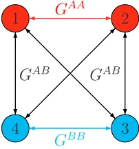
{1,2,3,4}, partitioned into two homogeneous groups, Π := {A, B} = {{1,2},{3,4}}. Each player is located at a vertex of a fully connected undirected graph,Γ, where edges represent a local interaction between the adjacent players (neighbours). Along edge (i, j), i < j, neighbours i and j interact via Gπ(i)π(j), where π(k) denotes the group to which player k belongs. Play is simultaneous. Utilities are the unweighted sum of payoffs earned with neighbours, where the same action, chosen from the common action set {a, b}, must be used with each.
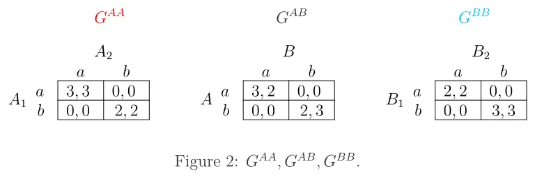
Figure1below shows the networkΓand the local interactions occurring along each edge. Vertices representing players in GroupAare coloured red, and those representing players in GroupB are coloured blue. Local interactions are also colour coded: within-group local interactions are the same colour as the two adjacent vertices, while across-group local interactions are black. Payoffs for each local interaction are as given in Figure 2. Note that in each local interaction, a player cares only about the actions chosen and not the opponent’s identity.
1 2
3 4
GAA
GBB
GAB
GAB
GAA GAB GBB
A1
A2
a b
a 3,3 0,0
b 0,0 2,2 A
B
a b
a 3,2 0,0
b 0,0 2,3 B1
B2
a b
a 2,2 0,0
b 0,0 3,3
Figure 2: GAA, GAB, GBB.
Now suppose that the above setting becomes the stage game of a repeated inter-action in discrete time. Players are boundedly rational and follow a simple updating rule. Specifically, whenever a player is afforded a revision opportunity, he takes a best-response against the current population profile. Letting (s1, s2, s3, s4) denote a partic-ular action profile, the only two (pure) equilibria to the one shot game are (a, a, a, a) and (b, b, b, b), denoted by (a,a) and (b,b) respectively. These equilibria are the only serious candidates for long run behaviour. The updating rule is the same for all players. It can be stated as: for tomorrow, take whatever action was used by at least two other players this period.
To discuss stochastic stability, we must specify a revision protocol (who is afforded a revision opportunity and when), and a model of mistakes (how players might deviate from the prescribed updating rule). As mentioned in the introduction, when limiting things to the two standard model of mistakes, there are three possible noisy dynamics, D1 - D3. It turns out that since both groups are the same size, the graph is fully connected, and payoffs (in a sense made precise in Neary (2011)) are “mirror image”, that in all three cases, stochastic stability selects both equilibria, (a,a) and (b,b).12
Remark 1 (Failure of lower hemicontinuity in payoffs). There are two important points related to perturbing the payoffs of the above game worth mentioning. The first is the failure of lower hemicontinuity of the selection correspondence with respect to payoffs when mistakes are logit. If the payoff that a particular group, say Group A, receives from coordinating on their preferred action is perturbed to 3+ε(ε>0). Then, Theorem
1shows that profile (a,a) is uniquely stochastically stable under the logit dynamics, and hence the selection correspondence is not continuous whenγA=γB = 3. Second, both
12Throughout this Section, dynamics D1 and D2 will agree on the selected outcome. The fully
dynamics D1 and D2 select both equilibria when payoffs are perturbed slightly. Since more than one equilibrium can be selected for an open set of parameters when errors are uniform, stochastic stability is really a refinement tool and not one of selection.
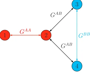
Now suppose that the original fully connected graph,Γ, is altered by removing edges (1,3) and (1,4). What is left is the subgraph ofΓ, ˆΓ, with the same vertex set and set of edges{(1,2),(2,3),(2,4),(3,4)}. This is depicted in Figure 3 below.
1 2
3
4 GAA
GAB
GAB
GBB
Figure 3: Network ˆΓ, a subnetwork ofΓ.
Assuming that whatever edges remain have the same local interaction played across them, the set of (pure) equilibria to this new game is the same as in the fully-connected case: (a,a) and (b,b) (this can be seen by noting that player 1 must coordinate with player 2). So, despite the fact that the network structure is now quite different and has lost its air of symmetry, the symmetric profiles are still the only candidate rest points of any best-response based dynamic.
Now I will compute the stochastically stable equilibria for each noisy dynamic. The divergence in prediction is quite striking. However, before getting to that, it makes sense to look at what the updating rule specifies for each player. With this information, it is then easy, but tedious, to perform a crude, but standard, “counting” argument to conclude which outcome(s) is (are) stochastically stable when mistakes are uniform. The updating rule for each player is as follows:
player 1: take whatever action player 2 took this period.
player 2: take whatever action was used by at least two of your neighbours this period.
Dynamics D1 & D2: Best-response dynamics with uniform mistakes
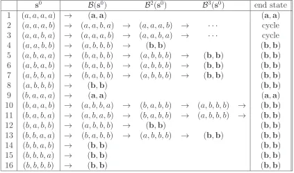
Computating the stochastically stable outcome for D1 is notationally far less cumber-some than for D2, and since they agree for this example I use only it. There are 24 = 16 states. Table1below lists each state, ordered lexicographically under the relationa < b, and examines where the best-reply dynamic terminates for each initial state, tracing the path by which it arrives there using the updating rules given above. Let s0 denote the initial state and B the best-reply dynamic. I write B2(·) = B!
B(·)"
for the 2-fold iteration of B, and so on. The successor state in a sequence follows a “→” symbol.
s0 B(s0) B2(s0) B3(s0) end state 1 (a, a, a, a) → (a,a) (a,a) 2 (a, a, a, b) → (a, a, b, a) → (a, a, a, b) → · · · cycle 3 (a, a, b, a) → (a, a, a, b) → (a, a, b, a) → · · · cycle 4 (a, a, b, b) → (a, b, b, b) → (b,b) (b,b) 5 (a, b, a, a) → (b, a, b, b) → (a, b, b, b) → (b,b) (b,b) 6 (a, b, a, b) → (b, a, b, b) → (a, b, b, b) → (b,b) (b,b) 7 (a, b, b, a) → (b, a, b, b) → (a, b, b, b) → (b,b) (b,b) 8 (a, b, b, b) → (b,b) (b,b) 9 (b, a, a, a) → (a,a) (a,a) 10 (b, a, a, b) → (a, b, b, a) → (b, a, b, b) → (a, b, b, b) → (b,b) 11 (b, a, b, a) → (a, b, a, b) → (b, a, b, b) → (a, b, b, b) → (b,b) 12 (b, a, b, b) → (a, b, b, b) → (b,b) (b,b) 13 (b, b, a, a) → (b, a, b, b) → (a, b, b, b) → (b,b) (b,b) 14 (b, b, a, b) → (b,b) (b,b) 15 (b, b, b, a) → (b,b) (b,b) 16 (b, b, b, b) → (b,b) (b,b)
Table 1: Evolution of B for each initial state.
Of the 16 strategy profiles, the only rest points of Bare the symmetric ones. States ‘1’ and ‘9’ lead to (a,a), states ‘2’ and ‘3’ form their own closed cycle, while the remaining 12 states all come to rest at (b,b)
To discuss how stochastically stable equilibria are computed when mistakes are uniform it is necessary to introduce a little bit of terminology.13 The deterministic
best-reply dynamic, B, induces a nonergodic Markov process, with transition matrix
13These techniques were first introduced to game theory in Foster and Young(1990) and are now
very standard. In this section I will be very informal and simply invoke a sufficient condition result
ofEllison (2000). These sufficient conditions are not always satisfied - see Section 5.2 ofNeary(2012)
PB, on the state space S. The process PB has three recurrent classes corresponding to the two rest points and the closed cycle of B: R1 = {(a,a)}, R2 = {(b,b)}, and
R3 ={(a, a, a, b),(a, a, b, a)}. All other states will transition with probability 1 to either (a,a) or (b,b), with the set that lead to each referred to as its basin of attraction.
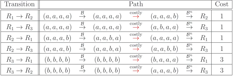
The cost between any two states s1 and s2, denoted c(s1,s2), is the number of simultaneous mistakes needed to transformB(s1) tos2. For the purpose of this example, all that is important is to examine “minimum cost paths” from each recurrent class to the basin of attraction of the other recurrent classes since from there the process can proceed “free of charge” to the equilibrium. Table 2 below displays a (not necessarily unique) minimum cost path and its cost for each pair of recurrent classes.
Table 2: Transition Costs
Transition Path Cost
R1 →R2 (a, a, a, a) B
→ (a, a, a, a) costly→ (a, a, a, b) →Bn R2 1
R1 →R3 (a, a, a, a) B
→ (a, a, a, a) costly→ (a, b, a, a) →Bn R3 1
R2 →R1 (a, a, a, b) B
→ (a, a, b, a) costly→ (a, a, a, a) →Bn R1 1
R2 →R3 (a, a, a, b) B
→ (a, a, b, a) costly→ (a, a, b, b) →Bn R3 1
R3 →R1 (b, b, b, b) B
→ (b, b, b, b) costly→ (b, a, a, a) →Bn R1 3
R3 →R2 (b, b, b, b) B
→ (b, b, b, b) costly→ (a, a, a, b) →Bn R3 3
From Table 2, a minimum cost path away from R3 = (b,b), is strictly more costly than any path leading to it. The radius-coradius result of Ellison (2000) is therefore applicable, and implies that (b,b) is the uniquely stochastically stable equilibrium.
Dynamic D3: Asynchronous learning with logit mistakes
In this case, a table like Table 1 above is not helpful since, (i) each state has multiple possible successors, and (ii) costly transitions are not of equal cost. Fortunately, a convenient shortcut is available. Since each local interaction of the Language Game is a potential game (Shapley and Monderer, 1996), the Language Game is as well (see Section4). With logit mistakes, the stochastically stable states are precisely those that maximise the potential (Theorem 1).
equilibrium. The reason for this is that payoffs are mirror image and there are the same number of within-group local interactions - so the global perspective of the potential function weights within-group edges equally. Thus, again Dynamic D3 selects both equilibria - in stark contrast to that with uniform mistakes. However, a similar state-ment as that made in Remark1holds again: if either group’s payoffs were increased by
ε as before, then uniform adoption of this group’s preferred action becomes uniquely stochastically stable. This statement is true even of GroupA.
3
The Model
3.1
Networks
A network is an undirected graphΓ = (N, E), where N ={1, . . . , N} denotes the set of vertices, and E ⊆ {(i, j)|i&=j ∈N } denotes the set of edges, such that (j, i) ∈ E
whenever (i, j) ∈ E.14 If (i, j) ∈ E, say that edge (i, j) has ends i and j, and that
vertices i and j are adjacent. I will abuse notation by writing E = {gij}i,j∈N, where
gij = 1, if i and j are adjacent, and 0 otherwise.
A networkΓ" = (N", E") is asubnetworkofΓ= (N, E), if bothN" ⊆N andE" ⊆E.
For any network Γ = (N, E), and for any two nonempty subsets, X, Y ⊆N, consider the set of edges with one end inXand the other inY,EXY :={(i, j)∈E|i∈X, j ∈Y}.
The subnetwork induced by a set of edges F ⊆E, that has edge set F and vertex set consisting of all vertices which lie at the end of at least one edge inF, is denotedΓ[F]. Similarly, the subnetwork ofΓ induced by a set of vertices C ⊆N, is denoted by Γ[C]
!
= (C, ECC)"
.
3.2
The Language Game
The Language Game is defined as the tuple L :=#N,Π,Γ, S,G$, where Π:={A, B} is a partition of N into nonempty groups A and B of sizes NA and NB respectively
(N = NA+NB); Γ := (N, E) is the path connected network15 on which the players
14The symbols⊆and⊂connote weak inclusion and strict inclusion respectively.
15A path is a sequence of distinct vertices such that each vertex is adjacent to the next in the
live;16 S :={a, b} is the action set common to all players; and G:=%
GAA, GAB, GBB&
is the collection oflocal interactions, whereGAAis the game that a player from GroupA
plays with a player from GroupA, etc. Payoffs for the local interactions are as follows,
GAA GBB
A1
A2
a b
a γA,γA 0,0
b 0,0 1−γA,1−γA B1
B2
a b
a 1−γB,1−γB 0,0
b 0,0 γB,γB
GAB
Ai
Bj
a b
a γA,1−γB 0,0
b 0,0 1−γA, γB
where γA,γB ∈ (1/2,1), so that, regardless of the opponent, Group A members always prefer to coordinate ona, while those in Group B prefer to coordinate on b.
The Language Game is a simultaneous move game. Since the focus is on dynamically stable outcomes, I assume that players do not randomise. Utilities are the unweighted sum of payoffs earned from interacting with neighbours, where the same action must be used with each. Players in a given group are differentiated only by the identity of those to whom they are connected. Local interactions are opponent-independent in that a player’s payoff depends only on the actions chosen and not the other player’s identity. Extending this, a player cares only about the number of his neighbours who choose the same action, and not who those neighbours are.
Define S:='Nj=1Sj with typical element s= (s1, . . . , sN). From the perspective of
some player j, an action profile, s ∈ S, can be viewed as (sj;s). Writing 1{·} for the
indicator function of event {·}, for typical players i ∈ A and k ∈ B, the utility from taking actions ∈S is given by,
16The network structure is assumedexogenous. This paper has nothing to say about how a particular
UA
i (si;s) :=γA1{si=a}
(
j#=i
gij1{sj=a}+ (1−γA)1{si=b}
(
j#=i
gij1{sj=b} (1)
UB
k (sk;s) := (1−γB)1{sk=a}
(
l#=k
gkl1{sl=a}+γB1{sk=b}
(
l#=k
gkl1{sl=b} (2)
In the Language Game, there are always at least two strict equilibria (the symmetric profiles), and possibly more depending on the strength of preferences (the values of
γA and γB) and the structure of the network. Equilibria where both actions appear are interesting when actions are interpreted as languages (or standards or operating systems). This implies the existence of more than one language existing in equilibrium - a feature not permitted in homogeneous agents models.
4
Dynamics and Potential
Now suppose the Language Game becomes the stage game of a repeated interaction. Time is discrete, begins at t= 0, and goes forever. Undiscounted utilities are received every period. At the beginning of a period, some subset of players is drawn from the population and each player in this set is afforded the opportunity to revise his current action. From here on I will refer to action profiles as “states” in “state space”S.
Any population dynamic with the above features induces a time-homogeneous non-ergodic Markov Process on state spaceS, with transition matrixP. By assuming that an agent may occasionally choose a suboptimal action, an ergodic Markov process, with transition matrixPε, that is “close to” the original processP, is generated. (Pεis
some-times called aperturbation of P.) Since Pε is ergodic, it possesses a unique stationary
distribution, µε. As shown by Foster and Young (1990) andYoung (1993),µε is “close
to” one of the (potentially) many stationary distributions ofP, µ# := lim ε↓0µε. The following is the main definition.
Definition 1. State s is stochastically stable, or selected, if µ#(s)>0, and uniquely so
if µ#(s) = 1. For the Language Game, denote this set of states by Ξ(L).
that could happen under P are still possible, however there are now additional transi-tions that could also happen - those that happen when a player accidentally chooses an action not prescribed by the learning rule. Thus, transitions allowed under Pε include
those that could happen underP, and some extra ones. While adding noise means that the system is always in flux, the now-noisy process spends the bulk of time localised around a subset of the equilibria - the stochastically stable ones.
Computing µ# is the objective. This is done by assigning a cost to every allowable
transition and then finding the minimum costs-tree. (The general procedure is sketched in AppendixA.) In this paper, computation ofµ# is quite different under each of the two
mistake parameterisations. The general procedure is used when mistakes are uniform; a convenient shortcut is available when mistakes are logit. I now describe each in turn.
4.1
Uniform Mistakes
Since transitions that can happen under Pε but not under P do so only seldom, they
can be thought of as having a cost associated with them. Transitions that could happen underP are deemed costless. Since mistakes happen with state-independent probability, a player choosing a mistaken action has a cost normalised to 1. Thus, if transitioning directly froms" tos""requires 4 players to make mistakes, then it is said to have a cost of 4. Clearly mistakes are required to occur in order to escape from equilibria. Intuitively, though it is not an entirely accurate statement, the more mistakes that are required to destabilise an equilibrium, the more likely that equilibrium is to be observed over time, i.e. be stochastically stable. (See Example 4 inNeary (2012) for a counterexample.)
4.2
Asynchronous Learning with Logit Mistakes
In this case, the likelihood of playing a particular action is exponentially related to its expected payoff, where again a player correctly forecasts the behaviour of others to remain unchanged. If the current population profile iss, and player i is selected, then player i chooses action s ∈ S according to the probability distribution pβi(s|s), where for any β>0,
pβi(s|s) :=
exp!
βUi(s;s) "
exp!
βUi(a;s) "
+ exp!
βUi(b;s)
" (3)
likelihood. Asβ → ∞, the response distribution as defined in (3) approaches that of a best-response. Thus, for any finite β, (3) defines a perturbation of the best-response. By combining the perturbed best-response dynamics for each player (assuming that β
is common across everyone), it is now the case thatµ# := lim
β→∞µβ.
Since mistakes happen with varying likelihood, the cost of each mistake is not equal and so normalisation is useless. This makes direct computation of µ# a difficult task.
But fortunately, given the particular structure of the Language Game, there is a very workable shortcut. The shortcut exploits the fact that the Language Game is a potential game (Shapley and Monderer,1996). A game is said to be apotential gameif the change in each player’s utility from choosing an action can be derived from a common function, referred to as the game’spotential function. Formally,
Definition 2. An N-person game G=#{Si}Ni=1,{Ui}Ni=1$ is a potential game if there exists a function ρ:S→R such that, for all i∈N, all s∈S, and all pairss"
i, s""i ∈Si,
we have that Ui(s"i;s)−Ui(s""i;s) =ρ(s"i;s)−ρ(s""i;s).
Local interactionsGAA, GAB, andGBBare potential games with respective potential
functions17 ρAA : S×S → R, ρAB : S ×S → R, and ρBB : S×S → R, where each
is defined as follows (forρAB, the first argument refers to the Group A player’s action,
and the second to the GroupB player’s action),
ρAA(a, a) =γA ρAA(a, b) = 0
ρAA(b, a) = 0 ρAA(b, b) = 1−γA
ρAB(a, a) =γA+ 1−γB ρAB(a, b) =γA
ρAB(b, a) = 1−γB ρAB(b, b) = 1 (4)
ρBB(a, a) = 1−γB ρBB(a, b) = 0
ρBB(b, a) = 0 ρBB(b, b) =γB
Since each local interaction is a potential game, by a straightforward result inNeary
(2011), the Language Game is itself a potential game, with potential function,ρ#, where
for any action profile s,
ρ#(s) := (
(ij)∈EAA i<j
ρAA(s
i, sj) + (
(ik)∈EAB i∈A, k∈B
ρAB(s
i, sk) + (
(hk)∈EBB h<k
ρBB(s
h, sk) (5)
The following result is straightforward but key. (It is a direct implication of a Theorem inNeary (2011), which itself is an extension of a result from Blume (1993).)
Theorem 1. For every β >0, Pβ has the unique stationary distribution, µβ, given by
µβ(s) = exp
!
βρ#(s)" )
s!∈Sexp
!
βρ#(s")" (6)
where ρ# is the potential function of L as defined in equation (5).
Furthermore, the stochastically stable states for a dynamic of asynchronous learning with logit mistakes,Ξ(L), are precisely those that maximise the potential function ρ#.
Computing the profiles that maximize the potential function ρ# can be reduced to
an integer programming problem as follows. Without loss of generality, identify {a, b}
with {0,1}. It is then the case that we can rewrite the potentials in (4) as follows, where, for anyi, j ∈A and h, k ∈B,
ρAA(si, sj) = (1−si)(1−sj)γA+sisj(1−γA)
ρAB(s
j, sk) = (1−sj)(1−sk)(γA+ 1−γB) + (1−sj)skγA+sj(1−sk)(1−γB) +sjsk1 ρBB(s
h, sk) = (1−sh)(1−sk)(1−γB) +shsk(γB)
Thus, the problem maxs∈Sρ#(s) can be reformulated as the following program,
max {s1,...,sN}∈{0,1}N
* (
i,j∈A i<j
gijρAA(si, sj) + (
i∈A,k∈B
gikρAB(si, sk) + (
h,k∈B h<k
ghkρBB(sh, sk) +
Since computation of stochastically stable equilibria amounts to weighting edges of the network in a maximal way, and that there are only three types of edges, it will prove useful to classify them.
An undirected graph, Γ = (N, E), is said to be bipartite if the vertex set can be split into two disjoint sets,N" and N"", such that no two vertices from the same set are
adjacent. The pair (N",N"") is known as the bipartition of Γ. In the Language Game,
Γ[EAB] is bipartite. While the bipartition need not be unique unless Γ[EAB] is path
connected, throughout the paper I will always assumeΓ[EAB] to be the bipartite graph !
(VA, VB), EAB"
, where VA ⊆ A and VB ⊆ B. This allows us to view the network Γ
asΓ[A]∪Γ[EAB]∪Γ[B].
It will also be important to count edges. Recall that for any network Γ = (N, E), and for any two nonempty subsets, X, Y ⊆N, the set of edges with one end in X and the other inY is given by EXY. Let e(X, Y) := |EXY| be the number of such edges.
The next section looks at the most commonly studied network structure - the fully connected network. Section 6 looks at arbitrary network structures, with particular emphasis on the across-group edges, EAB, and the effect they have on equilibrium
selection.18 My analysis completely ignores why such patterns might arise. Rather I
study the issue of equilibrium selection conditional on such a pattern existing.
5
The Fully Connected Network
When Γ is fully connected (gij = 1 for all i &= j), there are only 3 candidate profiles
for equilibria: {(a,a),(a,b),(b,b)}, where (a,b) is the profile where all of Group A
choose action a and all of Group B choose action b, etc. Profiles (a,a) and (b,b) are always strict equilibria; profile (a,b) is an equilibrium provided the ratios of preferred payoff to less preferred payoff are sufficiently large for each group.19 Behaviour at each
of these strategy profiles is said to begroup symmetric.
When the network is fully connected, there are essentially only two representative players, since at all strategy profiles, players in a given group face a similar strategic
18Previous versions of the paper examined two network structures that appear frequently in the
literature, stars and wheels.
19Precisely, it requires that (NA−1)γA≥NB(1−γA) and (NB−1)γB≥NA(1−γB). One must
problem.20 It is then useful to condense the state space, by viewing it as a lattice.
To illustrate this, consider the following example taken from Neary (2012).
Example 1. (NA, NB) = (10,5), (γA,γB) = (3/5,2/3),g
ij = 1 for all i&=j.
Figure4 below shows a condensed version of the state spaceS as an 11×6 lattice. The number of players in Group A using action a, taking values in {0, . . . ,10}, is on the horizontal-axis, and the number of Group B players using action a, taking values in{0, . . . ,5}, is on the vertical-axis. Each ‘state’ is depicted by a circle.
A large circle denotes an equilibrium. Corner states (0,0) and (NA, NB) are always
rest points, while corner state (NA,0) is also an equilibrium if the conditions of footnote 19are satisfied. For the parameters of this example, the only two equilibria are (0,0) and (10,5).
Figure 4 is also a preference map, with states colour-coded. The set of solid blue circles connotes states at which all players prefer action b. Solid red circles connote states at which all players prefer action a. At the states depicted by hollow circles, group preferences disagree - Group A players prefers a, while Group B players prefer
b.21 These sets are defined by equations (8) - (11) below.
Keeping in mind footnote21, Figure 4also depicts basins of attraction of the equi-libiria, where the basin of attraction of an equilibrium is the set of states from where there is positive probability of the unperturbed dynamics leading to that equilibrium. It is clear to which equilibrium the solid circles lead. The hollow circles are also colour coded: hollow red circles lead unambiguously to (10,5), since they must lead to the solid red circles; hollow black circles lead to both equilibria with positive probability. To un-derstand this last statement, consider state (4,5). If four Group B players are afforded revision opportunities successively before any Group A player is, then the dynamics will lead to state (4,2) from where they will unambiguously lead to (0,0); if two Group
Aplayers are the first to be afforded a revision opportunity, then after two periods the state will be (6,5) from where the terminal rest point is guaranteed to be (10,5). Note
20It is not correct to say that all players in a given group face the identical strategic problem,
since unless they are all currently using the same action, they will observe a different, though similar, distribution of actions in the population as a whole. Importantly however, while at most action profiles there are always two players in a given group who observe a different distribution of actions, their best-responses will typically coincide.
21Caveat: this last statement is not entirely accurate. At states in the set{(6,4),(7,3),(8,2),(9,1)},
~ s s s s s s s s s s s s s s s s s s s s s c c c c c c c c c c c c c c c c c c c c c c c c c c c c c s s s s s s s s s s s s s s s s ~ 0 1 2 3 4 5
0 1 2 3 4 5 6 7 8 9 10
Figure 4: Condensed State Space.
that this outcome is possible under asynchronous learning and independent inertia, but is impossible under the best-reply dynamic. Thus, under the best-reply dynamic all hollow states are uniquely in the basin of attraction of state (10,5).
5.1
Uniform Mistakes
In a companion paper,Neary (2012), I studied the fully connected setting in depth for the case where mistakes are uniform but where the revision protocol was purely deter-ministic. This was done so that the e↵ect ofgroup dynamism on equilibrium selection could be addressed, i.e. to answer the question, how would the groups’ relative reaction rates, that can also be interpreted as speed of learning, a↵ect long run outcomes? Ad-dressing such a question came at the cost of assuming that all players in a given group face the same population profile at all states. This is clearly not always accurate (see Footnotes20 and 21above).
As said before, computing stochastically stable equilibria with uniform mistakes amounts to computing paths of minimum cost from each equilibrium to the basins of attraction of the other equilibria. A path of minimal cost away from an equilibrium is equivalent to a path of shortest distance to a di↵erent basin of attraction. Some additional notation is required to analyse this formally.
any x∈R+, define ,x-:= min{n∈N|x≤n}. When a player is making a decision on what action to use, he considers the current distribution of actions in the population. Letna and nb denote the number of players in the population currently using actions
a and b respectively. Define the following,22
nA
a := min %
na ,
,UA(a;s)> UA(b;s) &
=,(1−γA)(N −1)-, (8)
nBa := min %
na ,
,UB(a;s)> UB(b;s) &
=,γB(N −1)-, (9)
nA
b := min %
nb ,
,UA(a;s)< UA(b;s) &
=,γA(N −1)-, (10)
nB
b := min %
nb ,
,UB(a;s)< UB(b;s) &
=,(1−γB)(N −1)- (11)
Thus, nA
a is the number of players currently taking action a for there to be at least
one player from GroupA to strictly prefer action a, etc.
There are two cases to consider, one where (a,b) is an equilibrium, and another where it is not.
5.1.1 Equilibrium Set is {(b,b),(a,a)}.
LetV!
(b,b)"
andV!
(a,a)"
denote basins of attraction for (b,b) and (a,a) respectively.
Theorem 2. Suppose the Equilibrium set is{(b,b),(a,a)}. Let τ∗
(b,b) and τ(∗a,a) denote
minimum costs-trees for (b,b) and (a,a) respectively. Then, 1. if (NA,0)&∈V!
(b,b)"
, then (a) Under noisy dynamic D1,
c(τ(∗a,a)) =n
A
a, (12)
c(τ(∗b,b)) =nAb; (13)
(b) Under noisy dynamic D2,
c(τ(∗a,a)) =nA
a, (14)
c(τ(∗b,b)) = max
%
nB
b , nAa −1 &
; (15)
22The values given are for generic parameters. Handling nongeneric parameters is tedious and does
2. if (NA,0)&∈V!
(a,a)"
, then (a) Under noisy dynamic D1,
cΨ(τωbb∗ ) =n B
b , (16)
cΨ(τωaa∗ ) =n B
a. (17)
(b) Under noisy dynamic D2,
cΨ(τωbb∗ ) =n B
b , (18)
cΨ(τωaa∗ ) = max %
nA a, N
B−nB
b + 1
&
. (19)
In each case, the set of stochastically stable states are those with the s-tree of mini-mum cost.
Let’s see how Theorem 2 applies. Consider Example 1. Since (NA,0)&∈ V!
(b,b)"
, we are in case1. Under both dynamics D1 andD2, the minimum cost (a,a)-tree,τ(∗a,a), has cost equal to 6. This is due to the fact that any of the states wherena= 6 will lead
to state (a,a). This will happen with certainty under D1, and with positive probability underD2.
Now consider the minimum cost (b,b)-tree, τ(∗b,b). Under noisy dynamic D1, 10 mistakes are required so that one of the blue states can be reached. However, under noisy dynamic D2, only 5 mistakes are required. Specifically, if 5 Group A players make mistakes (either sequentially with asynchronous learning or simultaneously with independent inertia) and accidentally choose action b, then the resulting state with be (5,5). From there, there is a positive probability of transitioning to state (5,0), from where the process will proceed with certainty to (b,b).
To summarise:
• Selected equilibrium under D1: (a,a)
• Selected equilibrium under D2: (b,b)
5.1.2 Equilibrium Set is {(b,b),(b,a),(a,a)}.
costly to transition from (a,b) to (b,b) via (a,a) rather than directly.
Theorem 3. Suppose the Equilibrium set is{(b,b),(b,a),(a,a)}. Let τ∗
(b,b), τ(∗a,b), and
τ∗
(a,a), denote minimum cost s-trees for (b,b), (b,a) and (a,a) respectively. Then,
cΨ(τ(∗b,b)) = min
#
nB
b + (n
A
b −N
B),(nB
a −N
A) + max%
nB b , N
A−nA
a −1
&$
(20)
cΨ(τ(∗a,b)) =nBb +n A
a (21)
cΨ(τ(∗a,a)) = min
#
nA
a + (n
B
a −N
A),(nA
b −N
B) + max%
nA a, N
B−nB
b −1
&$
(22)
The set of stochastically stable states are those with s-tree of minimum cost.
5.2
Logit Mistakes
By Theorem1, all we have to do is compute the potential at each of the group-symmetric profiles {(b,b),(b,a),(a,a)}. To help with computing these, the following facts are useful. The number of edges on any fully connected undirected graph with N vertices is !N
2
"
, and so, e(A, A) = !NA
2
"
and e(B, B) = !NB
2
"
. Furthermore, a bipartite graph
!
(X, Y), E"
is said to be fully connected if and only if gij = 1 for alli∈X and j ∈Y.
The number of edges on the fully connected bipartite graph Γ[EAB] is e(VA, VB) =
e(A, B) =NA×NB.
Using the expressions in (4), we get
ρ#!
(a,a)"
= !NA
2
"
·γA + (NA×NB)·(γA+ 1−γB) + !NB
2
"
·(1−γB)
ρ#!
(a,b)"
= !NA
2
"
·γA + (NA×NB)·γA + !NB
2
" ·γB ρ#!
(b,b)"
= !N2A"
·(1−γA) + (NA×NB)·1 + !NB
2
" ·γB
(23) where the first term on the right hand side of each equality is the potential due to edges
EAA, the second due to edges EAB, and the third due to edges EBB.
By Theorem1, the stochastically stable equilibria are those which maximizeρ#. For
(a,b) to be stochastically stable, it must be that
γA ≥ γ#
A := 1 2 + 1 2 NB
N −1 and γB ≥ γ
# B := 1 2 + 1 2 NA
N −1 (24)
From the omitted algebra, it is the conditionρ#!
(a,b)"
≥ρ#!
(a,a)"
lower bound ofγ#
B. It is intuitive that comparison of these two states yield a requirement
for a Group B player’s payoff, since obviously all GroupA players prefer (a,a).
Now let’s see how Theorem 1 applies to Example 1. By plugging in for parameters in the three expression in (23), we get that ρ#!
(a,a)"
= 77, ρ#!
(a,b)"
= 6323, and
ρ#!
(b,b)"
= 7423. Thus profile (a,a) is uniquely stochastically stable under noisy dynamicD3.
A natural question to ask is the relationship between equilibrium selection and Pareto-efficiency. This question was also addressed in Neary (2012). There it was shown that when the network is fully connected and dynamic D1 is considered that, i) an equilibrium may be Pareto-inefficient, but ii) a Pareto-inefficient equilibrium will never be selected. The following Theorem shows that this results carries over to the logit dynamic, D3.23
Theorem 4. Suppose the network is fully connected, and parameters are such that action profile (a,b) is an equilibrium. If under dynamic D3, (a,b) is stochastically stable, then it must be Pareto-efficient.
Theorem 4, whose proof is found in Appendix B, yields the first of the following relations (the second implication is a property of the stage game, not of dynamics, and appears in Theorem 6 of Neary (2012)):
stochastically stable under D3 ⇒Pareto-efficient ⇒ Equilibrium
While the reverse implications hold true for the symmetric profiles, they need not hold true for profile (a,b). To see this, suppose that NA=NB = 50 and let us vary payoffs.
When γA = γB = 0.55, we have that (a,b) is an equilibrium but not Pareto-Efficient. WhenγA =γB = 0.70, we have that (a,b) is Pareto-efficient (and hence an equilibrium) but not stochastically stable.
For the sake of intuition, two special cases are useful. The first supposes that payoffs are equal; the second supposes that the group sizes are equal.
1: γA=γB.
In this case, it can be shown that,ρ#!
(a,a)"
≥ρ#!
(b,b)"
⇐⇒ (2γA−1)-!NA
2
"
−
!NB
2
".
≥ 0. Given that 2γA >1, this holds only if !NA
2
"
≥ !NB
2
"
, which happens
23The symmetric profiles are always Pareto-efficient equilibria, so Theorem4is only concerned with
only if NA ≥ NB, i.e. if Group A is the bigger group. Thus, when payoffs are
mirrored, if one group has strictly more members than the other, the stochastically stable equilibrium cannot involve all players uniformly adopting the preferred outcome of the smaller group.24
2: NA =NB.
Here it can be shown that sign-ρ#!
(a,a)"
−ρ#!
(b,b)".
= sign/
γA−γB0
. Thus, if both groups are of equal size, the stochastically stable outcome will involve all players uniformly adopting the preferred outcome of the group with stronger preferences, unless bothγA≥γ#
A and γB ≥γB#.
To conclude this section, I briefly discuss the relationship between stochastically stable equilibria, and equilibrium profiles that maximise the sum of payoffs.25
Un-fortunately this criterion is only partially successful, even when the network is fully connected. When a symmetric profile is stochastically stable, it is not hard to show that it must maximise the sum of payoffs, but problems occur when profile (a,b) is stochastically stable. While profile (a,b) must be Pareto efficient if selected (Theo-rem 4), and thus a collective deviation by one group would lower their utilities, doing so would clearly raise the payoffs of those in the other group. Consider an example where NA = NB = 10, and γA = γB = 0.8. It can be checked that profile (a,b) is
stochastically stable, but that both symmetric profiles yield higher sum of payoffs.
6
Closely-knit Groups and Equilibrium Selection
If the groups are isolated from each other, it is clear what action each would like to coordinate on. The results ofPeski(2010) for the homogeneous agent model, show that in isolation a group will coordinate upon the locally risk-dominant action regardless of the network structure (provided, in the case that mistakes are uniform, that the network satisfies a mild density condition - in particular, that it does not have any star-like
substructures). Thus, decentralised play will lead to a desirable outcome when Pareto-efficiency coincides with risk dominance, and an undesirable outcome otherwise.
24In fact, a considerably stronger statement that applies to arbitrary networks is possible. When
payoffs are mirrored, if one group has strictly more within-group edges than the other group, then the stochastically stable equilibrium cannot involve all players uniformly adopting the preferred outcome of the group with fewer within-group edges.
Peski’s result can be interpreted negatively: from the perspective of a social en-gineer, it is not possible to implement a particular outcome by designing a network and simply letting people play. That is, varying network architecture has no affect on selection - risk dominance will ultimately prevail. A similar question can be asked for the Language Game (though it is not clear how risk-dominance ought be defined in a such a heterogeneous setting - see the discussion inNeary (2012)). In particular, what properties must a group’s subnetwork satisfy in order for all its members to adopt the preferred action in the long run? It is intuitive that agents in a given group must not only be well-connected internally, but also must not be overly-connected to those in the other group. The following definition, taken fromYoung(2001), provides a natural measure of intra-group connectedness relative to the other group.
Definition 3. Given a real number p ∈ (0,1), say that a subset of agents L ⊆ N is
p-closely-knit if,
∀Q⊆L, Q&=∅, e(Q, L)
e(Q, Q) +e(Q,N) ≥ p (25)
Close-knittedness is related to the concept of p-cohesiveness in Morris (2000).26 A
group is said to be p-cohesive if for each agent in the group, at least a fraction p of his connections are to those in the group (and hence at most a fraction 1−p of his connections are to those outside the group). By considering only singleton subsets, it is clear that a group of agents isp-cohesive whenever it is p-closely-knit, since for each singleton subset Q, the term e(Q, Q) in (25) is equal to zero. However, the reverse implication need not hold due to differences that arise when considering non-singleton subsets.
At first glance, it might seem unnatural that the term e(Q, Q) appears twice in the dominator (since, by definition it is also included in the term e(Q,N)), and hence one may want to consider a definition without it. However, the double counting of the e(Q, Q) term has a strategic interpretation that I now explain. Note that since
Q⊆L⊆N, we have thate(Q,N) =e(Q, L) +e(Q,N \L). Using this and rearranging
26Caveat: When normalising payoffs insymmetric binary coordination games, the literature often
assumes that the payofffrom thedesirable outcome is given by 1−pwherepis less than 0.5 (Morris,
2000). The reason for doing this, is that an agent then needs to see a fraction at least as great asp
expression (25) above, we have that for all nonemptyQ⊆L, it must be that
(1−p)e(Q, L)≥p!
e(Q, Q) +e(Q,N \L)"
(26)
Thus, for a group L to be closely knit, for any subset of the group, (1−p) times the number of edges between the subset and the group, must exceed p times the sum of edges between the subset and itself, and the subset and those outside the group. Again, this may seem a little mysterious until one supposes that those in L are defined by a common behaviour that they, and only they adopt. Expression (26) is then ‘counting’ edges in relative to the subset where behaviour is the same. Effectively it is considering what would happen if those in the subset Q collectively deviated from the action that defines the set L. In other words, given that the group L was defined by the behaviour of its agents, if those in subset Q now changed theirs, then they should no longer be considered part of L, and hence as outside of L. In a binary action game where actions are strategic complements, after a collective deviation, an agent inQ will now coordinate with those outside ofL but also with thoseQ(who also deviated). In other words, those in Q have now gone from coordinating with those in L to coordinating with those outside ofL (of which they are now a part).
With a purely deterministic dynamic like that considered byMorris(2000), a collec-tion of agents simultaneously adopting what is an inferior accollec-tion from the perspective of any individual, could not occur without some kind of external coordination device. But in the presence of perpetual mistakes there is always that possibility. In fact, it turns out that each GroupK ∈Π being (1−γK)-closely-knit is precisely the condition required for each group to coordinate upon their preferred action (and hence a complete failure to coordinate across the groups).
Theorem 5. Action profile(a,b)is stochastically stable under dynamicD3if and only if each Group K ∈Π is (1−γK)-closely knit.
Proof. The proof is contained in Appendix B.
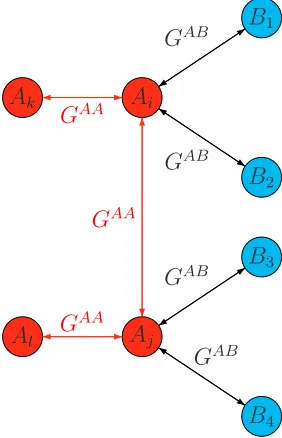
5, of particular importance are those Group A players who are connected to Group B
players, VA (players A
i and Aj in Figure 6). First of all, the inequality in (26) must
hold for all singleton sets Q = {Ai} ⊆ VA. So each individual player A
i ∈ VA must
have more connections to those in his own group than (1−γA)/γA times the number of connections to those inVB (whereVB denotes those in GroupB who are connected
to players at least one person from Group A). Note that for these singleton sets, this is just a restriction on individual behaviour, since if action a is not a best response for player Ai ∈ VA to the profile where all other Group A players take action a and all
Group B players take action b, then profile (a,b) is not even an equilibrium. (This is precisely Morris’ notion ofp-cohesive.)
However, unlike the concept ofp-cohesive, holding for all singleton subsets of VA is
insufficient for the inequality to hold for all Q ⊆ VA as Figure6 below demonstrates.
Agent Ai ∈ VA is adjacent to those in the set V1B = {B1, B2} ⊂ VB. Agent Ai is
also adjacent to agents Aj and Ak from A. Thus, by taking Q = {Ai}, the relevant
inequality holds for any value of γA given that γA > 1/2 > 1−γA. Similarly, agent
Aj ∈VA is adjacent to two agents from VB, those in V2B ={B3, B4}⊂VB. Note that
VB
1 ∩V2B =∅. Agent Aj is connected to agentsAi, and Al from Group A. So choosing
Q={Aj}, inequality (26) clearly holds. However, by choosing Q={Ai, Aj}, it is the
case that e(Q, VB) = 4, whereas e(Q, A\Q) = 2, and as such inequality (26) will only
hold forγA ∈[5/8,1) and not forγA∈(1/2,5/8).
Implicitly, the discussion above using Figure 6 shows that (a,b) must be robust tocoalitional deviations for agents in a given group if it is to be stochastically stable. Refinements of nash equilibrium requiring robustness to coalitional deviations have re-ceived much attention in the literature but, at least to my knowledge, their relationship to stochastically stable outcomes has so far been unexplored.27
The final result of the paper, Theorem6 below, provides necessary conditions for a symmetric profile to be stochastically stable.
Theorem 6. For a symmetric profile to be stochastically stable under dynamic D3, it
27Aumann (1959) introduced the notion of astrong equilibrium, where an equilibrium is robust to
unilateral and collective deviations. Bernheim, Peleg, and Whinston(1987) introducedcoalition-proof
equilibrium that is similar to strong equilibrium with the extra requirement that the deviation must
Ai
B1
B2
Aj
B3
B4
Ak
Al
GAA
GAB
GAB GAA
GAB
GAB GAA
Figure 5: Failure to coordinate across group.
must be the case that for each groupK ∈Π, and each nonempty subset Q⊆K, that
1−γK
2γK−1 ≥
e(Q, Q)
e(Q,N \Q) (27)
The proof of Theorem 6 is found in Appendix B. I will briefly discuss the intuition here. Condition (27) holds trivially for the group whose preferred symmetric profile is stochastically stable. For the less-content group, what the condition says is that the ratio of the payoff at this less-preferred symmetric profile to the payoff windfall (the payoff from their preferred equilibrium action minus their less preferred one) must exceed the number of internal edges within the subset Q relative to the number of edges from the subset Qto those outside it. Again, condition (27) effectively rules out profitable coalitional deviations by all subsets of the less-content group
7
Conclusion
ex-amination isBergin and Lipman(1996), who showed that for a given game and a given revision protocol (and a given learning dynamic), that any strict equilibrium can be rendered stochastically stable with an appropriately defined model of mistakes.28
How-ever, to my knowledge there are no games for which the uniform mistakes of KMR andYoung (1993) select different outcomes to the payoff-dependent (logit) mistakes of
Blume (1993). With the introduction of multiple populations in the Language Game, this immediately comes to the fore, and suggests that the answer to the original question is more subtle than first appeared. Furthermore, given that these two mistake models accord most with experimental evidence and also are those invoked most frequently, further investigation seems warranted.
In addition to individual mistakes, I have showed that equilibrium selection is not robust to the revision protocol. That is, for a given behavioural rule (myopic best-response) and a given model of mistakes (uniform mistakes), equilibrium selection can vary. As such, the modeller of a economic environment invoking stochastic stability as a selection criterion should be careful, and should justify what revision protocol best suits the situation. In a related paper,Lim and Neary (2013), a laboratory experiment is carried out in an attempt to distinguish between dynamics D1, D2, and D3, for the case that the network is fully connected.
Lastly, I have showed that equilibrium selection in the Language Game, a game where actions are strategic complements, is susceptible to network architecture. Unfor-tunately computing stochastically stable equilibria for such situations is difficult, with perhaps the major complicating issue, as it is with many games on arbitrary networks, being that there can be lots of equilibria. However, it is easily shown that the Language Game is a supermodular game, meaning that its equilibrium set must form a lattice (Vives,1990;Milgrom and Roberts,1990), and since there exist algorithms designed to compute equilibria in supermodular games (see for exampleEchenique(2007)), perhaps the problem is not as difficult as first appears.
28There are also many papers that show how by tweaking the stage game of the homogeneous
agent model, typically by complicating it slightly, risk-dominance need not be the prediction.
Canals and Vega-Redondo (1998) and Robson and Vega-Redondo (1996) vary the frequency with