The Thirty-Third AAAI Conference on Artificial Intelligence (AAAI-19)
EA-CG: An Approximate Second-Order
Method for Training Fully-Connected Neural Networks
Sheng-Wei Chen
HTC Research & HealthcareChun-Nan Chou
HTC Research & Healthcarejason.cn [email protected]
Edward Y. Chang
HTC Research & Healthcareedward [email protected]
Abstract
For training fully-connected neural networks (FCNNs), we propose a practical approximate second-order method includ-ing: 1) an approximation of the Hessian matrix and 2) a conju-gate gradient (CG) based method. Our proposed approximate Hessian matrix is memory-efficient and can be applied to any FCNNs where the activation and criterion functions are twice differentiable. We devise a CG-based method incorporating one-rank approximation to derive Newton directions for train-ing FCNNs, which significantly reduces both space and time complexity. This CG-based method can be employed to solve any linear equation where the coefficient matrix is Kronecker-factored, symmetric and positive definite. Empirical studies show the efficacy and efficiency of our proposed method.
Introduction
Neural networks have been applied to solving problems in several application domains such as computer vision (He et al. 2016), natural language processing (Hochreiter and Schmidhuber 1997), and disease diagnosis (Chang et al. 2017). Training a neural network requires tuning its model parameters using Backpropagation. Stochastic gradient de-scent (SGD), Broyden-Fletcher-Goldfarb-Shanno and one-step secant are representative algorithms that have been em-ployed for training in Backpropagation.
To date, SGD is widely used due to its low computational demand. SGD minimizes a function using the function’s first derivative, and has been proven to be effective for train-ing large models. However, stochasticity in the gradient will slow down convergence for any gradient method such that none of them can be asymptotically faster than simple SGD with Polyak averaging (Polyak and Juditsky 1992). Besides gradients, second-order methods utilize the curvature infor-mation of a loss function within the neighborhood of a given point to guide the update direction. Since each update be-comes more precise, such methods can converge faster than first-order methods in terms of update iterations.
For solving a convex optimization problem, a second-order method can always converge to the global minimum in much fewer steps than SGD. However, the problem of neural-network training can be non-convex, thereby suffer-ing from the issue of negative curvature. To avoid this issue,
Copyright c2019, Association for the Advancement of Artificial Intelligence (www.aaai.org). All rights reserved.
the common practice is to use the Gauss-Newton matrix with a convex criterion function (Schraudolph 2002) or the Fisher matrix to measure curvature since both are guaranteed to be positive semi-definite (PSD).
Although these two kinds of matrices can alleviate the is-sue of negative curvature, computing either the exact Gauss-Newton matrix or Fisher matrix even for a modestly-sized fully-connected neural network (FCNN) is intractable. In-tuitively, the analytic expression for the second derivative requires O(N2) computations if O(N) complexity is re-quired to compute the first derivative. Thus, several pioneer works (LeCun et al. 1998; Amari, Park, and Fukumizu 2000; Schraudolph 2002) have used different methods to approx-imate either matrix. However, none of these methods have been shown to be computationally feasible and fundamen-tally more effective than first-order methods as reported in (Martens 2010). Thus, there has been a growing trend towards conceiving more computationally feasible second-order methods for training FCNNs.
We outline several notable works in chronological or-der herein. Martens proposed a truncated-Newton method for training deep auto-encoders. In this work, Martens used an R-operator (Pearlmutter 1994) to compute full Gauss-Newton matrix-vector products and made good progress within each update. Martens and Grosse developed a block-diagonal approximation to the Fisher matrix for FC-NNs, called Kronecker-factored Approximation Curvature (KFAC). They derived the update directions by exploiting the inverse property of Kronecker products. KFAC features that its cost in storing and inverting the devised approxima-tion does not depend on the amount of data used to estimate the Fisher matrix. The idea is further extended to convo-lutional nets (Grosse and Martens 2016). Recently, Botev, Ritter, and Barber presented a block-diagonal approxima-tion to the Gauss-Newton matrix for FCNNs, referred to as Kronecker-Factored Recursive Approximation (KFRA). They also utilized the inverse property of Kronecker prod-ucts to derive the update directions. Similarly, Zhang et al. introduced a block-diagonal approximation of the Gauss-Newton matrix and used conjugate gradient (CG) method to derive the update directions.
sev-eral of these notable methods relying on the Gauss-Newton matrix face the essential limit that they cannot handle non-convex criterion functions playing an important part in some problems. Use robust estimation in computer vision (Stew-art 1999) as an example. Some non-convex criterion func-tions such as Tukey’s biweight function are robustness to outliers and perform better than convex criterion functions (Belagiannis et al. 2015). On the other hand, in order to de-rive the update directions, some of the methods utilizing the conventional CG method may take too much time, and the others exploiting the inverse property of Kronecker products may require excessive memory space.
To remedy the aforementioned issues, we propose a block-diagonal approximation of the positive-curvature Hes-sian (PCH) matrix, which is memory-efficient. Our proposed PCH matrix can be applied to any FCNN where the acti-vation and criterion functions are twice differentiable. Par-ticularly, our proposed PCH matrix can handle non-convex criterion functions, which the Gauss-Newton methods can-not. Besides, we incorporate expectation approximation into the CG-based method, which is dubbed EA-CG, to derive update directions for training FCNNs in mini-batch setting. EA-CG significantly reduces the space and time complexity of the conventional CG method. Our experimental results show the efficacy and efficiency of our proposed method.
In this work, we focus on deriving a second-order method for training FCNNs since the shared weights of convolu-tional layers lead to the difficulties in factorizing its Hes-sian. We defer tackling convolutional layers to our future work. We also focus on the classification problem and hence do not consider auto-encoders. Our strategy is that once a simpler isolated problem can be effectively handled, we can then extend our method to address more challenging issues. In summary, the contributions of this paper are as follows:
1. For curvature information, we propose the PCH matrix to improve the Gauss-Newton matrix for training FCNNs with convex criterion functions and overcome the non-convex scenario.
2. To derive the update directions, we devise effective EA-CG method, which does converge faster in terms of wall clock time and enjoys better testing accuracy than com-peting methods. Specially, the performance of EA-CG is competitive with SGD.
Truncated-Newton Method on Non-Convex
Problems
Newton’s method is one of the second-order minimization methods, and is generally composed of two steps: 1) com-puting the Hessian matrix and 2) solving the system of lin-ear equations for update directions. The truncated-Newton method applies the CG method with restricted iterations to the second step of Newton’s method. In this section, we first introduce the truncated-Newton method in the context of convex problems. Afterwards, we discuss the non-convex scenario of the truncated-Newton method and provide an important property that lays the foundation of our proposed PCH matrix.
Suppose we have a minimization problem
min
θ f(θ), (1)
wheref is a convex and twice-differentiable function. Since the global minimum is at the point that the first derivative is zero, the solutionθ∗can be derived from the equation
∇f(θ∗) = 0. (2)
We can utilize a quadratic polynomial to approximate Prob-lem 1 by conducting a Taylor expansion with a given point θj. Then, the problem turns out to be
min d f(θ
j
+d)≈f(θj) +∇f(θj)Td+1 2d
T
∇2f(θj
)d,
where ∇2f(θj) is the Hessian matrix of f at θj.
Af-ter applying the aforementioned approximation, we rewrite Eq. (2) as the linear equation
∇f(θj) +∇2f(θj)dj = 0. (3)
Therefore, the Newton direction is obtained via
dj =−∇2f(θj)−1∇f(θj),
and we can acquireθ∗by iteratively applying the update rule
θj+1=θj+ηdj,
whereηis the step size.
For non-convex problems, the solution to Eq. (2) reflects one of three possibilities: a local minimum θmin, a local
maximum θmax or a saddle point θsaddle. Some previous
works such as (Dauphin et al. 2014; Goldfarb et al. 2017; Mizutani and Dreyfus 2008) utilize negative curvature infor-mation to converge to a local minimum. Before illustrating how these previous works tackle the issue of negative cur-vature, we have to introduce a crucial concept that we can know the curvature information off at a given pointθ by analyzing the Hessian matrix∇2f(θ). On the one hand, the Hessian matrix of f at any θmin is positive semi-definite.
On the other hand, the Hessian matrices of f at anyθmax
andθsaddleare negative semi-definite and indefinite,
respec-tively. After establishing the concept, we can use the follow-ing property to understand how to utilize the negative curva-ture information to resolve the issue of negative curvacurva-ture.
Property 1. Letf be a non-convex and twice-differentiable function. With a given pointθj, we suppose that there ex-ist some negative eigenvalues {λ1, . . . , λs} for ∇2f(θj). Moreover, we take V = span({v1, . . . ,vs}), which is the
eigenspace corresponds to{λ1, . . . , λs}. If we take
g(k) =f(θj) +∇f(θj)Tv+1 2v
T∇2f(θj)v,
wherek∈ Rsandv =k1v1+. . .+ksvs, theng(k)is a
concave function.
According to Property 1, Eq. (3) may lead us to a lo-cal maximum or a saddle point if∇2f(θj
)has some neg-ative eigenvalues. In order to converge to a local mini-mum, we substitute Pos-Eig(∇2f(θj
))for∇2f(θj
Pos-Eig(A)is conceptually defined as replacing the negative eigenvalues ofAwith non-negative ones. That is,
Pos-Eig(A) =QT
γλ1 . ..
γλs λs+1
. ..
λn
Q,
whereγ is a given scalar that is less than or equal to zero, and{λ1, . . . , λs} and{λs+1, . . . , λn}are the negative and non-negative eigenvalues ofA, respectively. This refinement implies that the pointθj+1escapes from either local maxima or saddle points ifγ < 0. In case ofγ = 0, this refinement means that the eigenspace of the negative eigenvalues is ig-nored. As a result, we do not converge to any saddle point or local maximum. In addition, every real symmetric ma-trix can be diagonalized according to the spectral theorem. Under our assumptions,∇2f(θj
)is a real symmetric ma-trix. Thus, ∇2f(θj
)can be decomposed, and the function “Pos-Eig” can be realized easily.
When the number of variables in f is large, the Hes-sian matrix becomes intractable with respect to space com-plexity. Alternatively, we can utilize the CG method to solve Eq. (3). This alternative only requires calculating the Hessian-vector products rather than storing the whole Hes-sian matrix. Moreover, to save computation costs, it is desir-able to restrict the iteration number of the CG method.
Computing the Hessian Matrix
For second-order methods we must compute the curvature information, and we utilize the Hessian matrix to capture the curvature information in our work. However, the Hessian matrix for training FCNNs is intrinsically complicated and intractable. Recently, Botev, Ritter, and Barber presented the idea of block Hessian recursion, in which the diagonal blocks of the Hessian matrix can be computed in a layer-wise manner. As the basis of our proposed PCH matrix, we first establish some notation for training FCNNs and refor-mulate the block Hessian recursion with our notation. Then, we present the steps to integrate the approximation concept proposed by (Martens and Grosse 2015) into our reformula-tion.
Fully-Connected Neural Networks
An FCNN withk layers takes an input vectorh0i = xi,
wherexi is theith instance in the training set. For the ith
instance, the activation values in the other layers can be recursively derived from: hti = σ(Wthti−1 + bt), t = 1, . . . , k −1, where σ is the activation function and can be any twice differentiable function, and Wt and bt are the weights and biases in the tth layer, respectively. We further denote nt as the number of the neurons in the tth
layer, wheret = 0, . . . , k, and collect all the model param-eters including all the weights and biases in each layer as θ = (Vec(W1),b1, . . . ,Vec(Wk),bk), where Vec(A) =
[A·1]T [A·2]T · · · [A·n]T
T
. By following the nota-tion mennota-tioned above, we denote an FCNN output with k
layers ashki =F(θ|xi) =Wkhki−1+b k
.
To train this FCNN, we must decide a loss functionξthat can be any twice differentiable function. Training this FCNN can therefore be interpreted as solving the following mini-mization problem:
min θ
l
X
i=1
ξ(hki |yi)≡min θ
l
X
i=1
C(ˆyi|yi),
wherelis the number of the instances in the training set,yi is the label of theith instance,yˆ
i is softmax(h k
i), andCis
the criterion function.
Layer-wise Equations for the Hessian Matrix
For lucid exposition of the block Hessian recursion, we start by reformulating the equations of Backpropagation accord-ing to the notation defined in the previous subsection. Please note that we separate the bias terms (bt) from the weight terms (Wt) and treat each of them individually during back-ward propagation of gradients. The gradients of ξwith re-spect to the bias and weight terms can be derived from our reformulated equations in a layer-wise manner, similar to the original Backpropagation method. For theith instance, ourreformulated equations are as follows:
∇bkξi=∇hk
iξi
∇bt−1ξi=diag(h
(t−1)0 i )W
tT
∇btξi
∇Wtξi=∇btξi⊗h
(t−1)T i
whereξi = ξ(hki | yi), ⊗is the Kronecker product, and
h(it−1)0 = ∇zσ(z)|z=Wt−1ht−2
i +bt−1. Likewise, we strive to propagate the Hessian matrix ofξwith respect to the bias and weight terms backward in a layer-wise manner. This can be achieved by utilizing the Kronecker product and follow-ing the similar fashion above. The resultant equations for the
ithinstance are as follows:
∇2
bkξi=∇2hk i
ξi (4a)
∇2
bt−1ξi=diag(h
(t−1)0
i )W tT∇2
btξiWtdiag(h (t−1)0
i )
+diag(h(it−1)00(WtT∇btξi)) (4b)
∇2
Wtξi=(h
t−1
i ⊗h
(t−1)T i )⊗ ∇
2
btξi, (4c) where is the element-wise product, hh(it−1)00i
s
=
h
∇2
zσ(z)
z=Wt−1ht−2
i +bt−1
i
ss, and the derivative order of
∇2
Wtξi is column-wise traversal of W
t
. Moreover, it is worth noting that the original block Hessian recursion uni-fied the bias and weight terms, which is distinct from our separate treatment of these terms.
Expectation Approximation
and Barber 2017). The idea behind expectation approxima-tion is that the covariance between[hti−1⊗h(it−1)T]uvand
[∇btξi⊗ ∇btξiT]µν with given indices(u, v)and(µ, ν)is shown to be tiny and thus ignored due to computational ef-ficiency, i.e.,
Ei[[hti−1⊗h
(t−1)T
i ]uv·[∇btξi⊗ ∇btξiT]µν]
≈Ei[[hti−1⊗h(it−1)T]uv]·Ei[[∇btξi⊗ ∇btξiT]µν].
To explain this concept on our formulations, we define cov-t
as Ele-Cov((hti−1⊗h(it−1)T)⊗1nt,nt,1nt−1,nt−1⊗∇
2
btξi),
where ”Ele-Cov” is denoted as element-wise covariance, and 1u,v is the matrix whose elements are 1 in Ru×v, t = 1, . . . , k. With the definition of cov-tand our devised equations in the previous subsection, the approximation can be interpreted as follows:
Ei[∇2Wtξi] =EhhT
t−1⊗
Ei[∇2btξi] +cov-t
≈EhhTt−1⊗Ei[∇2btξi], (5)
where EhhTt−1=Ei[hit−1⊗h(it−1)T].
Botev, Ritter, and Barber also adopted expectation ap-proximation in their proposed method. Similarly, we inte-grate this approximation into our proposed layer-wise Hes-sian matrix equations, thereby resulting in the following ap-proximation equation:
Ei[∇2bt−1ξi]
≈Ei[diag(h(t−1)
0
i )W tT
Ei[∇2btξi]W
t
diag(h(t−1)
0
i )
+diag(h(it−1)00(WtT∇btξi))] =(WtTEi[∇2btξi]Wt)EhhT(t−1)
0
+Ei[diag(h(it−1)00(WtT∇btξi))]. (6)
where EhhT(t−1)0 =Ei[h(t−1) 0
i ⊗h
(t−1)0T
i ]. The difference
between the original and the approximate Hessian matrices in Eq. (6) is bounded by
Ele-Cov(W
tT
∇2btξiW
t ,h(t−1)
0
i ⊗h
(t−1)0T
i )
2
F
≤L4X
µ,ν
Var([WtT∇2
btξiW
t
]µν), (7)
whereLis the Lipschitz constant of activation functions. For example,LReLUandLsigmoidare1and0.25, respectively.
Deriving the Newton Direction
Now we present a computationally feasible method to train FCNNs with Newton directions. First, we explain the ways to construct a PCH matrix. Based on PCH matrices, we pro-pose an efficient CG-based method incorporating the expec-tation approximation to derive Newton directions for mul-tiple training instances, which we call EA-CG. Finally, we provide an analysis of the space and time complexity for EA-CG.
PCH Matrix
Based on our layer-wise equations in the previous section and the integration of expectation approxima-tion, we can construct block matrices that vary in size and are located at the diagonal of the Hessian ma-trix. We denote this block-diagonal matrix Ei[∇2θξi] as
diag(Ei[∇2W1ξi],Ei[∇2b1ξi], . . . ,Ei[∇2Wkξi],Ei[∇2bkξi]). Please note that Ei[∇2θξi] is a block-diagonal Hessian
matrix and not the complete Hessian matrix. According to the explanation for the three possibilities of update directions in aforementioned section, Ei[∇2θξi] is
re-quired to be modified. Thus, we replace Ei[∇2θξi] with
diag(Ei[∇[2W1ξi],Ei[∇d2b1ξi], . . . ,Ei[∇[2Wkξi],Ei[∇d2bkξi]) and denote the modified result asEi[∇c2
θξi], where
Ei[∇d2
bkξi] =Pos-Eig(Ei[∇2hk i
ξi]) (8a)
Ei[∇\2bt−1ξi] =(W
tT Ei[∇d2
btξi]W
t)EhhT(t−1)0
(8b)
+Pos-Eig(diag(Ei[hi(t−1)00(WtT∇btξi)]))
Ei[∇[2Wtξi] =EhhTt−1⊗Ei[∇d2
btξi]. (8c)
We callEi[∇c2θξi]the block-diagonal approximation of
pos-itive curvature Hessian (PCH) matrix. Any PCH matrix can be guaranteed to be PSD, which we explain in the following.
In order to showEi[∇c2
θξi]is PSD, we have to show that
for any t, both Ei[∇d2
btξi] and Ei[∇[2Wtξi] are PSD. First,
we consider the block matrixEi[∇2hk i
ξi]that is ank bynk
square matrix in Eq. (8a). If the criterion functionC(ˆyi |yi)
is convex, Ei[∇2hk i
ξi] is a PSD matrix. Otherwise, we de-compose the matrix and replace the negative eigenvalues. Fortunatelynk is usually not very large, soEi[∇2hk
i
ξi]can
be decomposed quickly1 and modified to a PSD matrix
Ei[∇d2
hk i
ξi]. Second, suppose thatEi[∇d2
btξi] is a PSD
ma-trix, then(WtTEi[∇d2
btξi]W
t)EhhT(t−1)0
is PSD.
Con-sequently, the negative eigenvalues ofEi[∇d2
btξi]stems form the diagonal part diag(Ei[h(t−1)
00
i (W tT∇
btξi)]), so we take the Pos-Eig function for this diagonal part in Eq. (8b). Third, because the Kronecker product of two PSD matrices
is PSD, it impliesEi[∇[2Wtξi]is PSD.
Solving Linear Equation via EA-CG
After obtaining a PCH matrixEi[∇c2θξi], we derive the
up-date direction by solving the linear equation
((1−α)Ei[∇c2θξi] +αI)dθ=−Ei[∇θξi], (9)
where 0 < α < 1 anddθ = [dTW1dbT1· · ·dTWkdTbk]T. Here, we use the weighted average ofEi[∇c2θξi]and an
iden-tity matrixIbecause this average turns the coefficient matrix
1
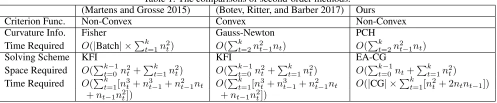
Table 1: The comparisons of second-order methods. (Martens and Grosse 2015) (Botev, Ritter, and Barber 2017) Ours
Criterion Func. Non-Convex Convex Non-Convex
Curvature Info. Fisher Gauss-Newton PCH
Time Required O(|Batch| ×Pk
t=1n 2
t) O(
Pk
t=2n 2
t−1nt) O(P k t=2n
2
t−1nt)
Solving Scheme KFI KFI EA-CG
Space Required O(Pk−1
t=0n 2
t+
Pk
t=1n 2
t) O(
Pk−1
t=0 n 2
t+
Pk
t=1n 2
t) O(
Pk−1
t=0 nt+P k t=1n
2
t)
Time Required O(Pk
t=1[n3t+nt3−1+n2t−1nt O(
Pk
t=1[n3t+n3t−1+n2t−1nt O(|CG| ×
Pk
t=1[n2t+ 2ntnt−1]) +nt−1n2t]) +nt−1n2t])
of Eq. (9) that is PSD to positive definite and thus makes the solutions more stable. Due to the essence of diagonal blocks, Eq. (9) can be decomposed as
((1−α)Ei[∇d2
btξi] +αI)dbt =−Ei[∇btξi] (10a) ((1−α)Ei[∇[2Wtξi] +αI)dWt =−Vec(Ei[∇Wtξi]),
(10b)
for t = 1, . . . , k. To solve Eq. (10a), we attain the solu-tions by using the CG method directly. For Eq. (10b), storing
Ei[∇[2Wtξi]is not an efficient way, so we apply the equation
(CT ⊗A)Vec(B) = Vec(ABC) and Eq. (5) to have the Hessian-vector product with a given vector Vec(P):
Ei[∇[2Wtξi]Vec(P)
=Vec(Ei[∇d2
btξi]·P·Ei[hti−1⊗h
(t−1)T
i ]) (11a)
≈Vec(Ei[∇d2
btξi]·P·Ei[hti−1]⊗Ei[h
(t−1)T
i ]). (11b)
Based on Eq. (11a), we derive the Hessian-vector
prod-ucts ofEi[∇[2Wtξi]viaEi[∇d2
btξi], thereby reducing the space
complexity of storing the curvature information. Further-more, applying the CG method becomes much more effi-cient with Eq. (11b), which we call EA-CG. The details are elaborated in the following subsections.
Analysis of Space Complexity
By considering the devised method in aforementioned sub-section, we analyze the required space complexity to store the distinct types of the curvature information. The origi-nal Newton’s method requires space to storeEi[∇2θξi], so
that its space complexity is O([Pk
t=1nt−1(nt + 1)]2). If we consider the PCH matrixEi[∇c2θξi], the space
complex-ity turns out to be O(Pk
t=1[(nt−1nt)2+n2t]). According
to Eq. (11a), it is not necessary to store Ei[∇[2Wtξi]
any-more becauseEi[∇d2
btξi]is sufficient to derive the solution to Eq. (9) with the CG method. Thus, the space complexity is reduced toO(Pk
t=1n2t).
Analysis of Additional Time Complexity
In this subsection, we elaborate on the additional time com-plexity introduced in our proposed method. In contrast to the SGD, our method contributes more computation to the
training process of FCNNs. The extra computation mainly originates from two portions of our method: the propa-gation of the curvature information and the computation of EA-CG method. To propagate the curvature informa-tion, we are required to perform the matrix-to-matrix prod-ucts twice, which is more computationally expensive than propagating gradients. The time complexity of propagat-ing the curvature information with Eq. (6) can be estimated as O(Pk
t=1[nt−1nt(nt−1+nt)]). We also have the extra cost involved in applying EA-CG method. The complexity of EA-CG method mainly stems from the Hessian-vector products Eq. (11b). Regarding Eq. (11b), we must conduct the matrix-vector products twice and the vector-vector outer products once in order to acquire the Hessian-vector prod-uct. Thus, the time complexity pertaining to the truncated-Newton method isO(|CG|×Pk
t=1[nt(2nt−1+nt)]), where |CG|is the number of iterations of EA-CG method.
Related Works
In this section, we elaborate on the differences between our work and two closely related works using the notation estab-lished in the previous sections.
Martens and Grosse developed KFAC by considering the FCNNs with the convex criterion and non-convex activa-tion funcactiva-tions. KFAC utilized (Ei[ ˜Fi] +αI) where F˜i is
the Fisher matrix (for any training instancexi) to measure
the curvature and used the Khatri-Rao product to rewriteF˜i,
which yields the following equation:
[ ˜Fi]µν = (h µ−1
i ⊗h
(µ−1)T
i )⊗(∇bνξi⊗ ∇bνξiT). Since it is difficult to find the inverse of(Ei[ ˜Fi]+αI), KFAC
substitutes a block-diagonal matrixFˆi for F˜i and thus has
the formulation:
Ei[ ˆFit] =Ei[(h t−1
i ⊗h
(t−1)T
i )⊗(∇btξi⊗ ∇btξTi )]
≈Ei[hti−1⊗h
(t−1)T
i ]⊗Ei[∇btξi⊗ ∇btξiT], wheret = 1, . . . , k. To derive(Ei[ ˆFit] +αI)−1efficiently,
KFAC comes up with the approximation
(Ei[ ˆFit] +αI)−1≈(Ht)−1⊗(Gt)−1, (12)
where (Ht)−1 = (
Ei[hti−1 ⊗ h
(t−1)T i ] + πt
√ αI)−1, (Gt)−1= (
Ei[∇btξi⊗ ∇btξTi ] + ( √
0 500 1000 1500 2000 2500 3000 3500 time(sec)
0.0 0.5 1.0 1.5 2.0
training loss
Fisher-KFI Fisher-CG GN-KFI GN-CG PCH-KFI PCH-CG SGD
0 500 1000 1500 2000 2500 3000 3500
time(sec) 10
15 20 25 30 35 40 45
test accuracy (%)
Fisher-KFI Fisher-CG GN-KFI GN-CG PCH-KFI PCH-CG SGD
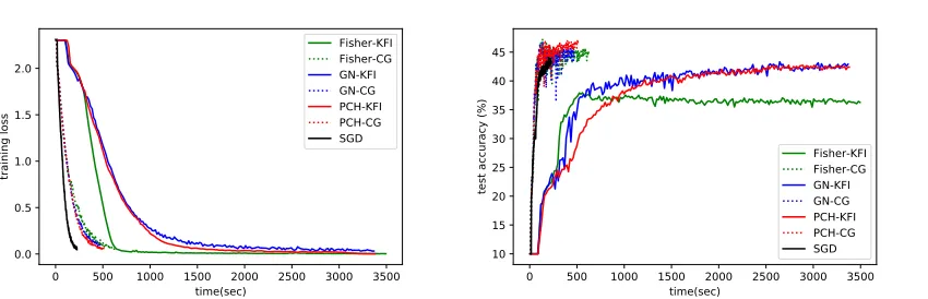
Figure 1: Comparison of different curvature information and solving methods for the convex criterion function “cross-entropy” on “Cifar-10”.
0 1000 2000 3000 4000
time(sec) 0.0
0.5 1.0 1.5 2.0
training loss
Fisher-KFI Fisher-CG GN-KFI GN-CG PCH-KFI PCH-CG SGD
0 1000 2000 3000 4000
time(sec) 10
15 20 25 30 35 40 45
test accuracy (%)
Fisher-KFI Fisher-CG GN-KFI GN-CG PCH-KFI PCH-CG SGD
Figure 2: Comparison of different curvature information and solving methods for the convex criterion function “cross-entropy” on “ImageNet-10”.
the update directions of KFAC can be acquired via the fol-lowing equation:
ˆ
dWt=−((Ht)−1⊗(Gt)−1)·Vec(Ei[∇Wtξi]) =−Vec((Gt)−1Ei[∇Wtξi](Ht)−1),
and we refer this type of inverse methods as Kronecker-Factored Inverse (KFI) methods in this paper. In contrast, we derive the update directions by applying EA-CG method. Moreover, KFAC uses the Fisher matrix, while we use the PCH matrix.
Based on the discussion of the FCNNs with convex cri-terion functions and piecewise linear activation functions, Botev, Ritter, and Barber developed KFRA. As a result, the diagonal term disappears in Eq. (4b). Thus, the Gauss-Newton matrix becomes no different from the Hessian ma-trix. KFRA also employs KFI method, and hence the update direction of KFRA can be derived from
˜
dWt =−Vec(( ˜Gt)−1Ei[∇Wtξi](Ht)−1), where( ˜Gt)−1= (
Ei[GN(∇2btξi)] + ( √
α/πt)I)−1, and GN
stands for Gauss-Newton matrix. The method of deriving the update directions is again different between KFRA and our work. In addition, KFRA still works under the non-convex activation functions, but it exists the difference be-tween Gauss-Newton matrix and Hessian matrix.
Table 1 highlights the three main components of these two related works and our method. As shown in Table 1, KFRA cannot handle non-convex criterion functions due to the cur-vature information they utilized. The Gauss-Newton matrix becomes indefinite if the criterion function is non-convex. Note that the difference between the original and approx-imated matrices always exists in Eq. (12) if Ei[ ˆFit]is not
diagonal. Moreover, the time complexity of KFI method is similar to EA-CG method.
Experimental Evaluation
Our empirical studies aim to examine not only three dif-ferent types of curvature information including the Fisher, Gauss-Newton and PCH matrices, but also the two solving methods, i.e., KFI and EA-CG methods, in terms of train-ing loss and testtrain-ing accuracy. We encompassed SGD with momentum as the baseline and fixed its momentum to0.9. For better comparison, we considered FCNNs with either convex or non-convex criterion functions and conducted our experiments2 on the image datasets that comprise Cifar-10
2
0 25 50 75 100 125 150 175 200 epoch
0.0 0.5 1.0 1.5 2.0
training loss
Fisher-KFI Fisher-CG GN-KFI GN-CG PCH-KFI PCH-CG SGD
0 25 50 75 100 125 150 175 200
epoch 10
15 20 25 30 35 40 45
test accuracy (%)
Fisher-KFI Fisher-CG GN-KFI GN-CG PCH-KFI PCH-CG SGD
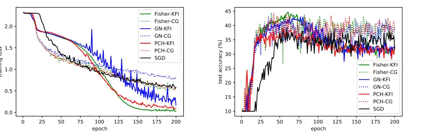
Figure 3: Comparison of different curvature information and solving methods for the convex criterion function “cross-entropy” on “Cifar-10”.
0 25 50 75 100 125 150 175 200
epoch 0.0
0.5 1.0 1.5 2.0
training loss
Fisher-KFI Fisher-CG GN-KFI GN-CG PCH-KFI PCH-CG SGD
0 25 50 75 100 125 150 175 200
epoch 10
15 20 25 30 35 40 45
test accuracy (%)
Fisher-KFI Fisher-CG GN-KFI GN-CG PCH-KFI PCH-CG SGD
Figure 4: Comparison of different curvature information and solving methods for the convex criterion function “cross-entropy” on “ImageNet-10”.
(Krizhevsky and Hinton 2009) and ImageNet-103. The net-work structures are “3072-1024-512-256-128-64-32-16-10” and “150528-1024-512-256-128-64-32-16-10” for Cifar-10 and ImageNet-10, respectively. For the PCH matrices, we explored two possible scenarios of Eq.(8b): 1) taking the ab-solute values of the diagonal part, i.e.,γ = −1and 2) ap-plyingmax(x,0)function to the diagonal part, i.e.,γ = 0. The first and second scenarios of the PCH matrices are sep-arately dubbed PCH-1 and PCH-2. Since PCH-1 and PCH-2 produced the similar results of training loss and testing ac-curacy, we only reported PCH-1 in the corresponding fig-ures below for the sake of simplicity. In all of our experi-ments, we used sigmoid as the non-convex activation func-tion of FCNNs and trained the networks with 200 epochs, i.e., seeing the entire training samples 200 times. Fur-thermore, we utilized “Xavier” initialization method (Glo-rot and Bengio 2010) and performed the grid search on learning rate = [0.05,0.1,0.2],|Batch| = [100,500,1000]
andα= [0.01,0.02,0.05,0.1]. Regarding EA-CG method, we have to determine two hyper-parameters that control its stopping conditions. One is the maximal iteration number, max|CG|; the other is the constant of the related error bound,
3
We randomly choose ten classes from the ImageNet (Deng et al. 2009) dataset.
CG. Thus, we also performed the grid search on max|CG|=
[5,10,20,50] and CG = [10−10,10−5,10−2,10−1].
Fi-nally, to further investigate the different types of curvature information, we calculate the errors caused by approximat-ing the true Hessian in a layer-wise fashion.
Convex Criterion
In the first type of experiments, we examined the perfor-mance of different second-order methods. According to the prior section, the differences between these second-order methods originate from two parts. The first part is the curva-ture information, e.g., the Fisher matrixFiˆ in KFAC, and the other is the solving method for the linear equations. In these experiments, we used cross-entropy as the convex criterion function.
It is noteworthy that the original KFI method runs out of GPU memory for ImageNet-10 because the dimension of the features (n0) in ImageNet-10 is too high, which conforms with our analysis in Table 1. Thus, we utilized
H1≈
Ei[h0i]⊗Ei[h
0T i ] +π1
√
αI (13)
0 500 1000 1500 2000 2500 3000 3500 time(sec)
0.40 0.45 0.50 0.55 0.60
training loss
Fisher-KFI Fisher-CG PCH-KFI PCH-CG SGD
0 500 1000 1500 2000 2500 3000 3500
time(sec) 10.0
12.5 15.0 17.5 20.0 22.5 25.0 27.5 30.0
test accuracy (%) Fisher-KFI
Fisher-CG PCH-KFI PCH-CG SGD
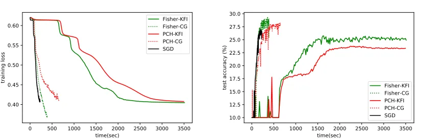
Figure 5: Comparison of different curvature information and solving methods for the non-convex criterion function “Eq. (14)” on “Cifar-10”. The Gauss-Newton matrix is removed from this figure since it is not PSD in this type of experiments.
0 1000 2000 3000 4000
time(sec) 0.40
0.45 0.50 0.55 0.60
training loss
Fisher-KFI Fisher-CG PCH-KFI PCH-CG SGD
0 1000 2000 3000 4000
time(sec) 10.0
12.5 15.0 17.5 20.0 22.5 25.0 27.5
test accuracy (%) Fisher-KFIFisher-CG
PCH-KFI PCH-CG SGD
Figure 6: Comparison of different curvature information and solving methods for the non-convex criterion function “Eq. (14)” on “ImageNet-10”. The Gauss-Newton matrix is removed from this figure since it is not PSD in this type of experiments.
Wall Clock Time As shown in Figure 1, EA-CG method converges faster with respect to wall clock time and has bet-ter performance of testing accuracy than KFI method for Cifar-10. The runtime behavior adheres to Table 1. We also notice that the different types of curvature information with EA-CG method have the similar performance. In contrast, KFI method using the Fisher matrix converges faster than using the other two types of matrices. For ImageNet-10, Figure 2 exhibits that EA-CG and KFI methods take al-most the same amount of time for200epochs. Besides, as shown in Figure 2, KFI method has lower training loss but may suffer from the overfitting issue. Please note that we applied Eq (13) to the first layer of the neural network for KFI method. Otherwise, the original KFI method ran out of GPU memory for ImageNet-10. However, applying this ap-proximation reduces the memory usage of KFI method but expedites KFI method accordingly.
It is worth noting that second-order methods performed comparable to SGD in Figure 2, but the phenomenon is com-pletely different in Figure 1. This is because the image sizes of Cifar-10 and ImageNet-10 are varied. The image size of ImageNet-10 is224×224×3, and hence propagating the gradients of the weights backward is much more expensive than it in Cifar-10 whose image size is32×32×3. Based
on this premise, the extra cost of propagating our proposed PCH where only the Hessian of the bias terms is required to propagate is comparatively low. Similarly, the cost of solv-ing the update directions is comparatively low.
Epoch As shown in Figure 3, KFI method provides a pre-cise descent direction of each epoch, so the training loss decreases faster in terms of epochs. In contrast, Figure 1 shows KFI method converges slower in terms of wall clock time, which varied with different implementation. We argue that we have already done our best effort to implement KFI method by using the inverse function in PyTorch. As shown in either Figure 1 or Figure 3, EA-CG method has the better results of testing accuracy for Cifar-10. For ImageNet-10, the results of Figure 4 are consistent with the results of Fig-ure 2. Thus, we do not repeat the same narrative here.
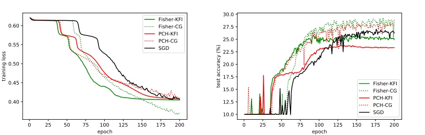
Non-Convex Criterion
In order to demonstrate our capability of handling non-convex criterion functions, we designed the second type of experiments. In these experiments, we considered the fol-lowing criterion function:
C( ˆyi|yi) = 1 1 +eδ(yT
iyˆi−)
0 25 50 75 100 125 150 175 200 epoch
0.40 0.45 0.50 0.55 0.60
training loss
Fisher-KFI Fisher-CG PCH-KFI PCH-CG SGD
0 25 50 75 100 125 150 175 200
epoch 10.0
12.5 15.0 17.5 20.0 22.5 25.0 27.5 30.0
test accuracy (%) Fisher-KFI
Fisher-CG PCH-KFI PCH-CG SGD
Figure 7: Comparison of different curvature information and solving methods for the non-convex criterion function “Eq. (14)” on “Cifar-10”. The Gauss-Newton matrix is removed from this figure since it is not PSD in this type of experiments.
0 25 50 75 100 125 150 175 200
epoch 0.40
0.45 0.50 0.55 0.60
training loss
Fisher-KFI Fisher-CG PCH-KFI PCH-CG SGD
0 25 50 75 100 125 150 175 200
epoch 10.0
12.5 15.0 17.5 20.0 22.5 25.0 27.5
test accuracy (%) Fisher-KFIFisher-CG
PCH-KFI PCH-CG SGD
Figure 8: Comparison of different curvature information and solving methods for the non-convex criterion function “Eq. (14)” on “ImageNet-10”. The Gauss-Newton matrix is removed from this figure since it is not PSD in this type of experiments.
where we fixδ= 5and= 0.2. This criterion function im-plies that the upper bound of the loss function exists. Apart from the criterion function, we followed the same settings as those used in the first type of experiments. Note that the Gauss-Newton matrix is not PSD if the criterion function of training FCNNs is non-convex. Thus, we excluded the Gauss-Newton matrix from this comparison and focused on comparing the other two types of matrices with either EA-CG or KFI methods.
Wall Clock Time For Cifar-10, Figure 5 shows that EA-CG method outperforms KFI method in terms of both train-ing loss and testtrain-ing accuracy. But the Fisher matrix with EA-CG method has the best performance. For ImageNet-10, Figure 6 shows that EA-CG method surpasses KFI method regarding training loss. But the performance of EA-CG and KFI methods is hard to distinguish by the testing accuracy.
Epoch As shown in Figure 7, for Cifar-10, the perfor-mance of EA-CG and KFI methods is hard to distinguish by the convergence speed of training loss in terms of epochs. But the Fisher matrix with EA-CG method has the best training loss in Figure 7. Regarding testing accuracy, EA-CG method has the better performance than KFI method for this type of experiments. For ImageNet-10, Figure 8 shows that EA-CG method surpasses KFI method regarding
train-Table 2: Layer-wise errors between each of the approximate Hessian matrices and the true Hessian for the convex crite-rion function “cross-entropy” on “Cifar-10”.
Fisher GN PCH-1 PCH-2
Layer-1 0.0071 0.0057 0.0036 0.0043 Layer-2 0.0470 0.0212 0.0237 0.0228 Layer-3 0.1140 0.0220 0.0238 0.0165 Layer-4 0.0726 0.0207 0.0119 0.0085 Layer-5 0.0397 0.0130 0.0086 0.0066 Layer-6 0.0219 0.0107 0.0093 0.0071 Layer-7 0.0185 0.0176 0.0132 0.0106 Layer-8 0.0251 0.0000 0.0000 0.0000 Total 0.1535 0.0446 0.0402 0.0330
ing loss, which is consistent with Figure 6. However, the performance of EA-CG and KFI methods is hard to distin-guish by the testing accuracy, and the PCH matrix using KFI method has the best testing accuracy.
Comparison with the True Hessian
fur-ther examine the difference between the true Hessian and the approximate Hessian matrices such as the Fisher matrix. Here, we measure the difference in the errors that is elabo-rated as follows. Given thetth layer and the model
parame-tersθ, the error is defined as
Ei[∇g
2
btξi]− |Ei[∇2btξi]|
F,
where∇g2
btξistands for the approximate Hessian matrix, and
|Ei[∇2
btξi]|is to take the absolute values of the eigenvalues
ofEi[∇2btξi], which we follow (Dauphin et al. 2014). The results are shown in Table 2 where each value is de-rived from averaging the errors of the initial parametersθ0 to the parametersθs−1that are updatedstimes. Table 2 re-flects that the errors are not accumulated with layers for any approximate Hessian matrix. This observation is important for KFRA and ours since both methods derive the curvature information by approximating the Hessian layer-by-layer re-cursively. The “Total” row of Table 2 also indicates that our proposed PCH-1 and PCH-2 are closer to the true Hessian than the Fisher and Gauss-Newton matrices.
Concluding Remarks
To achieve more computationally feasible second-order methods for training FCNNs, we developed a practical ap-proach, including our proposed PCH matrix and devised EA-CG method. Our proposed PCH matrix overcomes the problem of training FCNNs with non-convex criterion func-tions. Besides, EA-CG provides another alternative to effi-ciently derive update directions in this context. Our empiri-cal studies show that our proposed PCH matrix can compete with the state-of-the-art curvature approximation, and EA-CG does converge faster and enjoys better testing accuracy than KFI method. Specially, the performance of our pro-posed approach is competitive with SGD. As future work, we will extend the idea to work with convolutional nets.
References
Amari, S.-I.; Park, H.; and Fukumizu, K. 2000. Adaptive method of realizing natural gradient learning for multilayer perceptrons. Neural Computation12(6):1399–1409. Belagiannis, V.; Rupprecht, C.; Carneiro, G.; and Navab, N. 2015. Robust optimization for deep regression. In Proceed-ings of the IEEE International Conference on Computer Vi-sion, 2830–2838.
Botev, A.; Ritter, H.; and Barber, D. 2017. Practical gauss-newton optimisation for deep learning. In International Conference on Machine Learning, 557–565.
Chang, E. Y.; Wu, M.-H.; Tang, K.-F. T.; Kao, H.-C.; and Chou, C.-N. 2017. Artificial intelligence in xprize deepq tricorder. In Proceedings of the 2Nd International Work-shop on Multimedia for Personal Health and Health Care, MMHealth ’17, 11–18. New York, NY, USA: ACM. Dauphin, Y. N.; Pascanu, R.; Gulcehre, C.; Cho, K.; Gan-guli, S.; and Bengio, Y. 2014. Identifying and attacking the saddle point problem in high-dimensional non-convex op-timization. InAdvances in neural information processing systems, 2933–2941.
Deng, J.; Dong, W.; Socher, R.; Li, L.; Li, K.; and Fei-Fei, L. 2009. Imagenet: A large-scale hierarchical image database. In2009 IEEE Conference on Computer Vision and Pattern Recognition, 248–255.
Glorot, X., and Bengio, Y. 2010. Understanding the diffi-culty of training deep feedforward neural networks. In Teh, Y. W., and Titterington, M., eds.,Proceedings of the Thir-teenth International Conference on Artificial Intelligence and Statistics, volume 9 ofProceedings of Machine Learn-ing Research, 249–256. Chia Laguna Resort, Sardinia, Italy: PMLR.
Goldfarb, D.; Mu, C.; Wright, J.; and Zhou, C. 2017. Using negative curvature in solving nonlinear programs. Compu-tational Optimization and Applications68(3):479–502. Grosse, R., and Martens, J. 2016. A kronecker-factored approximate fisher matrix for convolution layers. In Inter-national Conference on Machine Learning, 573–582. He, K.; Zhang, X.; Ren, S.; and Sun, J. 2016. Deep resid-ual learning for image recognition. InProceedings of the IEEE conference on computer vision and pattern recogni-tion, 770–778.
Hochreiter, S., and Schmidhuber, J. 1997. Long short-term memory.Neural computation9(8):1735–1780.
Krizhevsky, A., and Hinton, G. 2009. Learning multiple lay-ers of features from tiny images. Technical report, Citeseer. LeCun, Y.; Bottou, L.; Orr, G. B.; and M¨uller, K.-R. 1998. Efficient backprop. InNeural networks: Tricks of the trade. Springer. 9–50.
Martens, J., and Grosse, R. 2015. Optimizing neural networks with kronecker-factored approximate curvature. In International Conference on Machine Learning, 2408– 2417.
Martens, J. 2010. Deep learning via hessian-free optimiza-tion. In Proceedings of the 27th International Conference on Machine Learning (ICML-10), 735–742.
Mizutani, E., and Dreyfus, S. E. 2008. Second-order stage-wise backpropagation for hessian-matrix analyses and inves-tigation of negative curvature. Neural Networks21(2):193– 203.
Pearlmutter, B. A. 1994. Fast exact multiplication by the hessian.Neural computation6(1):147–160.
Polyak, B. T., and Juditsky, A. B. 1992. Acceleration of stochastic approximation by averaging. SIAM Journal on Control and Optimization30(4):838–855.
Schraudolph, N. N. 2002. Fast curvature matrix-vector prod-ucts for second-order gradient descent. Neural computation 14(7):1723–1738.
Stewart, C. V. 1999. Robust parameter estimation in com-puter vision.SIAM review41(3):513–537.