Communication-efficient Sparse Regression
Jason D. Lee [email protected]
Marshall School of Business University of Southern California Los Angeles, CA 90089
Qiang Liu [email protected]
Department of Computer Science Dartmouth University
Hanover, NH 02714
Yuekai Sun [email protected]
Department of Statistics University of Michigan Ann Arbor, MI 48109
Jonathan E. Taylor [email protected]
Department of Statistics Stanford University Stanford, CA 94305
Editor:Zhihua Zhang
Abstract
We devise a communication-efficient approach to distributed sparse regression in the high-dimensional setting. The key idea is to average “debiased” or “desparsified” lasso esti-mators. We show the approach converges at the same rate as the lasso as long as the dataset is not split across too many machines, and consistently estimates the support un-der weaker conditions than the lasso. On the computational side, we propose a new parallel and computationally-efficient algorithm to compute the approximate inverse covariance re-quired in the debiasing approach, when the dataset is split across samples. We further extend the approach to generalized linear models.
Keywords: Distributed Sparse Regression, Averaging, Debiasing, lasso, high-dimensional statistics
1. Introduction
Explosive growth in the size of modern datasets has fueled interest in distributed statistical learning. For examples, we refer to Boyd et al. (2011); Dekel et al. (2012); Duchi et al. (2012); Zhang et al. (2013) and the references therein. The problem arises, for example, when working with datasets that are too large to fit on a single machine and must be distributed across multiple machines. The main bottleneck in the distributed setting is usually communication between machines/processors, so the overarching goal of algorithm design is to minimize communication costs.
c
In distributed statistical learning, the simplest and most popular approach isaveraging: each machine forms a local estimator ˆθk with the portion of the data stored locally, and a
“master” averages the local estimators to produce an aggregate estimator: ¯θ= m1 Pm k=1θˆk.
Averaging was first studied by Mcdonald et al. (2009) for multinomial regression. They derive non-asymptotic error bounds on the estimation error that show averaging reduces the variance of the local estimators, but has no effect on the bias (from the centralized solution). In follow-up work, Zinkevich et al. (2010) studied a variant of averaging where each machine computes a local estimator with stochastic gradient descent (SGD) on a random subset of the dataset. They show, among other things, that their estimator converges to the centralized estimator.
More recently, Zhang et al. (2013) studied averaged empirical risk minimization (ERM). They show that the mean squared error (MSE) of the averaged ERM decays likeO N−12+
m N
, where m is the number of machines and N is the total number of samples. Thus, so long asm.√N , the averaged ERM matches the N−12 convergence rate of the centralized ERM. Even more recently, Rosenblatt and Nadler (2014) studied the optimality of averaged ERM in two asymptotic settings: N → ∞,m, pfixed andp, n→ ∞, pn →µl∈(0,1), where
n = Nm is the number of samples per machine. They show that in the n → ∞, p fixed setting, the averaged ERM is first-order equivalent to the centralized ERM. However, when p, n→ ∞,the averaged ERM is suboptimal (versus the centralized ERM).
We develop a divide and conquer approach to statistical learning. In the high-dimensional setting, regularization is essential. The key idea is to average debiased ordesparsified reg-ularized M-estimators. Under suitable conditions, it is possible to show that the local debiased estimators are asymptotically normal. thus the averaged estimator delivers the same statistical performance as the computationally infeasible centralized M-estimator.
Formally, we show that the error of the averaged estimator decomposes into aOeP √1
N
asymptotically normal term and a remainder term. As long as m . √
N
slogp, wheres is the
sparsity of the unknown regression coefficients, the reminder term is asymptotically negli-gible. Thus the averaged estimator converges at the same rate as a centralized estimator. Further, the averaged estimator is model selection consistent under a weak minimum signal strength condition. In the following section, we review the theoretical properties of the lasso and debiased lasso and describe our contributions more formally.
2. A divide-and-conquer approach to sparse regression
To keep things simple, we focus on sparse linear regression. Consider the sparse linear model
y=Xβ∗+,
where the rows ofX∈Rn×pare predictors, and the components ofy ∈Rnare the responses.
To keep things simple, we assume
(A1) the predictors x ∈ Rp are independent σx-subgaussian random vectors with whose
(A2) the regression coefficients β∗ ∈ Rp are s-sparse, i.e. all but s components of β∗ are zero;
(A3) the components of the noise are independent, mean zero σy-subgaussian random
variables.
Given the predictors and responses, the lasso estimates β∗ by
ˆ
β:= arg min
β∈Rp
1
2nky−Xβk 2
2+λkβk1.
There is a well-developed theory of the lasso that says, under suitable assumptions on X, the lasso estimator ˆβ is nearly minimax optimal(e.g. see Hastie et al. (2015), Chapter 11 for an overview). More precisely, under some conditions on n1XTX, the MSE of the lasso estimator is roughly slogn p, which is the minimax rate.
2.1 Background on the lasso and debiasing
However, the lasso estimator is also biased1. Since averaging only reduces variance, not bias, we gain (almost) nothing by averaging the biased lasso estimators. That is, it is possible to show if we naively averaged local lasso estimators, the MSE of the averaged estimator is of the same order as that of the local estimators. The key to overcoming the bias of the averaged lasso estimator is to “debias” the lasso estimators before averaging.
The debiased lasso estimator by Javanmard and Montanari (2013a) is
ˆ
βd:= ˆβ+ 1 nΘˆX
T(y−Xβˆ), (1)
where ˆβ is the lasso estimator and ˆΘ ∈ Rp×p is an approximate inverse to ˆΣ = n1XTX. Intuitively, the debiased lasso estimator trades bias for variance. The trade-off is obvious when ˆΣ is non-singular: setting ˆΘ = ˆΣ−1 gives the ordinary least squares (OLS) estimator (XTX)−1XTy.
Another way to interpret the debiased lasso estimator is a corrected estimator that com-pensates for the bias incurred by shrinkage. By the optimality conditions of the lasso, the correction term n1XT(y−Xβˆ) is a subgradient of λk·k1 at ˆβ. By adding a term propor-tional to the subgradient of the regularizer, the debiased lasso estimator compensates for the bias incurred by regularization. The debiased lasso estimator has previously been used to perform inference on the regression coefficients in high-dimensional regression models. We refer to the papers by Javanmard and Montanari (2013a); van de Geer et al. (2013); Zhang and Zhang (2014); Belloni et al. (2011) for details.
The choice of ˆΘ in the correction term is crucial to the performance of the debiased estimator. Javanmard and Montanari (2013a) suggest forming ˆΘ row by row: thej-th row of ˆΘ is the optimum of
minimize
θ∈Rp θ
TΣˆθ
subject to kΣˆθ−ejk∞≤δ.
(2)
The parameterδ should large enough to keep the problem feasible, but as small as possible to keep the bias (of the debiased lasso estimator) small. As we shall see, when the rows of
X are subgaussian, setting δ ∼ lognp12
is usually large enough to keep (2) feasible.
Definition 1 (Generalized coherence) GivenX∈Rn×p,let Σ =ˆ 1
nXTX.The
general-ized coherence betweenΣˆ and Θ∈Rp×p is
GC( ˆΣ,Θ) = maxj∈[p]kΣΘˆ Tj −ejk∞.
The preceding definition is a generalization of the usual notion of coherence as it appears in the compressed sensing literature. Assume the columns of X are normalized so that kxjk2 = 1, and Θ = I. The diagonal entries of ˆΣΘ−I vanish. Thus GC( ˆΣ,Θ) is the largest off diagonal entry of ˆΣ, which is the largest inner product between columns of X:
1
nmaxi6=j
eTi XTXej
. We recognize the preceding quantity as the coherence of X.
Lemma 2 (Javanmard and Montanari (2013a)) Under (A1), when 16κσx4n > logp,
the event
EGC( ˆΣ) :=nGC( ˆΣ,Σ−1)≤ √8 c1
√
κσ2xlogp n
12o
occurs with probability at least 1−2p−2 for some c1>0,whereκ:= λλmax(Σ)min(Σ) is the condition number of Σ.
As we shall see, the bias of the debiased lasso estimate is of higher order than its variance under suitable conditions on ˆΣ.In particular, we require ˆΣ to satisfy therestricted eigenvalue (RE) condition.
Definition 3 (RE condition) For any S ⊂[p],let
C(S) :={∆∈Rp | k∆Sck
1 ≤3k∆Sk1}. We say Σˆ satisfies the RE condition on the cone C(S) when
∆TΣ∆ˆ ≥µlk∆Sk22
for some µl>0 and any ∆∈ C(S).
The RE condition requires ˆΣ to be positive definite on C(S). When the rows of X ∈ Rn×p are i.i.d. Gaussian random vectors, Raskutti et al. (2010) show there are constants µ1, µ2 >0 such that
1 nkX∆k
2
2 ≥µ1k∆k 2 2−µ2
logp n k∆k
2
1 for any ∆∈R
p
Lemma 4 (Rudelson and Zhou (2013)) Under (A1), if n >4000˜sσ2xlog Cp˜s
and p > ˜
s, where ˜s:=s+ 25920κs=C0s, the event
ERE(X) =n∆TΣ∆ˆ ≥ 1
2λmin(Σ)k∆Sk 2
2 for any∆∈ C(S)
o
occurs with probability at least 1−2e−
n
4000σx4,where C and C0 are universal constants.
Proof The lemma is a consequence of Rudelson and Zhou (2013), Theorem 6. In their notation, we set δ= √1
2, k0 = 3 and bound maxj∈[p]kAejk 2
2 and K(s0, k0,Σ 1
2) by λmax(Σ) and λmin(Σ)−
1 2.
When the RE condition holds, the lasso and debiased lasso estimators are consistent for a suitable choice of the regularization parameterλ.The parameterλshould be large enough to dominate the “empirical process” part of the problem: 1nXTy
∞,but as small as possible
to reduce the bias incurred by regularization. As we shall see, setting λ∼σy lognp
12
is a good choice.
Lemma 5 Under (A3),
1 nkX
Tk
∞≤maxj∈[p]( ˆΣj,j)
1 2σy
3 logp
c2n
12
with probability at least 1−ep−2 for any (non-random) X ∈Rn×p.
When ˆΣ satisfies the RE condition andλis large enough, Negahban et al. (2012) show that the lasso is consistent.
Lemma 6 (Negahban et al. (2012)) If in addition to (A2) and (A3),
1. Σˆ satisfies the RE condition onC(supp(β∗)) with constant µl
2. 1nkXTk∞≤λ,
kβˆ−β∗k1≤ 3 µl
sλ and kβˆ−β∗k2 ≤ 3 µl
√ sλ.
When the lasso estimator is consistent, the debiased lasso estimator is also consistent. Further, it is possible to show that the bias of the debiased estimator is of higher order than its variance. Similar results by Javanmard and Montanari (2013a); van de Geer et al. (2013); Zhang and Zhang (2014); Belloni et al. (2011) are the key step in showing the asymptotic normality of the (components of) the debiased lasso estimator. The result we state is essentially Javanmard and Montanari (2013a), Theorem 2.3.
Lemma 7 If in addition to (A2) and (A3),
1. Σˆ satisfies the RE condition onC(supp(β∗)) with constant µl
3. ( ˆΣ,Θ)ˆ has generalized incoherence δ,
the debiased lasso estimator has the form
ˆ
βd=β∗+ 1 n
ˆ
ΘXT+ ˆ∆,
where k∆kˆ ∞≤ 3µδ
lsλ.
Lemma 7, together with Lemmas 5 and 2, shows that the bias of the debiased lasso estimator is of higher order than its variance. In particular, settingλandδ to be the order of the upper bounds on infΘ∈Rp×pGC( ˆΣ,Θ) and 1
nkX Tk
∞given by Lemmas 5 and 2 gives
a bias termk∆kˆ ∞ that isOP slogn p
.By comparison, the variance term n1kΘˆXTk∞ is the
maximum ofp subgaussian random variables with mean zero and variances ofO(1),which
is O lognp 1
2. Thus the bias term is of higher order than the variance term as long as n&s2logp.
Corollary 8 If in addition to the conditions of Lemma 6,
1. ( ˆΣ,Θ)ˆ has generalized incoherence δ0 lognp 1 2,
2. λ= maxj∈[p]( ˆΣj,j)
1
2σy 3 logp
c2n
12 ,
k∆kˆ ∞≤
3√3 √
c2
δ0maxj∈[p]( ˆΣj,j)
1 2 µl
σy
slogp n .
The rest of the paper is organized as follows. In the subsequent section, we describe a divide-and-conquer approach to sparse regression and derive its theoretical properties. We show that
1. the averaged estimator converges at the same rate as the communication-intensive centralized lasso estimator. In particular, a thresholded version of the averaged esti-mator attains the same estimation rate as the centralized lasso estiesti-matorkβ¯ht−β∗k2.
slogp N
12
, and only requires one round of communication.
2. a thresholded version of the averaged estimator is model selection consistent as long as
the minimum signal strength is at least logNp 1
2. We remark that the model selection consistency result does not require X to obey an irrepresentability condition, which the centralized lasso does require.
Although the divide-and-conquer approach is communication efficient, it is costly in terms of floating point operations. The parallel runtime of debiasing is roughly equivalent to the cost of evaluating p lasso estimators, due to computation of ˆΘ. In the rest of this section, we describe a more sophisticated approach to debiasing: each machine debiases mp, instead of allp, regression coefficients. Thus the parallel runtime of the more sophisticated approach is roughly mtimes smaller than that of a naive approach.
the averaged debiased estimator outperforms averaging local lasso estimates, and performs as well as the centralized lasso. Section 5 generalizes our approach from least-squares to generalized linear models such as logistic regression.
Finally in Section 7, we show the optimality of our estimator in terms of the amount of communication, and rounds of communication using recent work on communication lower bounds. We also provide a comparison of the average debiased estimator and the centralized lasso estimator. The parallel runtime of the averaging debiased estimator is only larger than the centralized lasso by a constant multiplicative factor.
2.2 Averaging debiased lassos
Recall the problem setup: we are given N samples of the form (xi, yi) distributed across m
machines:
X=
X1 .. . Xm
, y =
y1 .. . ym
.
Thek-th machine has local predictorsXk∈Rnk×p and responsesyk ∈Rnk.To keep things
simple, we assume the data is evenly distributed, i.e. n1=· · ·=nk=n= Nm.Theaveraged
debiased lasso estimator (for lack of a better name) is
¯ β= 1
m
m
X
k=1 ˆ βkd= 1
m
m
X
k=1 ˆ
βk+ ˆΘkXkT(yk−Xkβˆk)
, (3)
We begin by studying the error of the ¯β in the`∞ norm.
Lemma 9 Suppose the local sparse regression problem on each machine satisfies the con-ditions of Corollary 8, that is when m≤p,
1. {Σˆk}k∈[m] satisfy the RE condition on C(supp(β∗)) with constant µl,
2. {( ˆΣk,Θˆk)}k∈[m] have generalized incoherence cGC lognp
12
,
3. λ1 =· · ·=λm=cΣσy 3 logc2np
12
.
Then
kβ¯−β∗k∞≤cσy
cΩlogp
N
12
+cGCcΣ µl
σy
slogp n
with probability at least1−ep−1,wherec >0is a universal constant,cΩ:= maxj∈[p], k∈[m](( ˆΘkΣˆkΘˆTk)j,j)
and cΣ:= maxj∈[p],k∈[m](( ˆΣk)j,j)
1 2.
Lemma 10 hints at the performance of the averaged debiased lasso. In particular, we note the first term is O logNp12
, which matches the convergence rate of the centralized
estimator. When n is large enough, slogn p is negligible compared to logNp12
, and the error
isO logNp12
.
Lemma 10 Under (A1), (A2), and (A3), when m < p, p >s˜,
1. n >max
4000˜sσx2log(Cps˜ ),8000σ4xlogp, c3
1 max{σ 2
x, σx}logp ,
2. λ1 =· · ·=λm= maxj∈[p],k∈[m](( ˆΣk
j,j)
1
2σy 3 logp
c2n
12 ,
3. δ1 =· · ·=δm = √8c1
√
κσx2 lognp 1
2 and form {Θˆ
k}k∈[m] by (2), kβ¯−β∗k∞≤c
σy
max
j∈[p]Σ−j,j1logp
N
12
+ √
κmaxj∈[p](Σj,j)
1 2 λmin(Σ)
σx2σy
slogp n
with probability at least 1−(8 +e)p−1 for some universal constant c >0.
The averaged debiased lasso has one serious drawback versus the lasso: ¯β is usually dense. The density of ¯β detracts from the intrepretability of the coefficients and makes the estimation error large in the `2 and `1 norms. To remedy both problems, we threshold the averaged debiased lasso:
HTt( ¯β)←β¯j·1{|β¯j|≥t},
STt( ¯β)←sign( ¯βj)·max{|β¯j| −t,0}.
As we shall see, both hard and soft-thresholding give sparse aggregates that are close toβ∗ in`2 norm.
Lemma 11 As long ast >kβ¯−β∗k∞, β¯ht:= HTt( ¯β) satisfies
1. kβ¯ht−β∗k∞≤2t,
2. kβ¯ht−β∗k2 ≤2√2st,
3. kβ¯ht−β∗k1 ≤2√2st.
The analogous result also holds for β¯st := STt( ¯β).
Proof By the triangle inequality,
kβ¯ht−β∗k∞≤ kβ¯ht−β¯k∞+kβ¯−β∗k∞
≤t+β¯−β∗
∞
≤2t.
Since t > β¯−β∗
∞, β¯jht = 0 whenever βj∗ = 0. Thus ¯βht is s-sparse and ¯βht −β∗ is
2s-sparse. By the equivalence between the `∞ and `2,`1 norms, kβ¯ht−β∗k2≤2
√ 2st,
kβ¯ht−β∗k1≤2√2st. The argument for ¯βst is similar.
Theorem 12 Under the conditions of Lemma 10, hard-thresholdingβ¯atσy
4 max
j∈[p]Σ −1
j,jlogp
c2N
12
+
48√6
√
c1c2
√
κmaxj∈[p](Σj,j)
1 2
λmin(Σ) σx2σyslogn p gives
1. kβ¯ht−β∗k∞.P σy
max
j∈[p]Σ−j,j1logp
N
12
+
√
κmaxj∈[p](Σj,j)
1 2
λmin(Σ) σ 2
xσyslogn p,
2. kβ¯ht−β∗k2 .P σy
max
j∈[p]Σ−j,j1slogp
N
12
+
√
κmaxj∈[p](Σj,j)
1 2
λmin(Σ) σ 2
xσys
3 2 logp
n ,
3. kβ¯ht−β∗k1 .P σy
max
j∈[p]Σ−j,j1s2logp
N
12
+
√
κmaxj∈[p](Σj,j)
1 2
λmin(Σ) σ 2
xσys
2logp
n .
Remark 13 By Theorem 12, when m . s2logn p, the variance term is dominant and the convergence rates given by the theorem simplify:
1. kβ¯ht−β∗k∞.P logNp
12
,
2. kβ¯ht−β∗k2 .P slogN p
1
2,
3. kβ¯ht−β∗k1 .P s2logN p12
.
The convergence rates for the centralized lasso estimatorβˆare identical (modulo constants):
1. kβˆ−β∗k∞.P logNp
12
,
2. kβˆ−β∗k2.P slogN p
12
,
3. kβˆ−β∗k1.P s
2logp
N
1
2.
The estimator β¯ht matches the convergence rates of the centralized lasso in `1, `2, and `∞ norms. Furthermore, β¯ht can be evaluated in a communication-efficient manner by a
one-shot averaging approach.
Corollary 14 Under the conditions of Lemma 10, further assume
1. m. s2logn p,
2. β-min: |βj∗|& logNp12
for any j∈supp(β∗).
Then supp( ¯βht) = supp(β∗).
Proof As long as we threshold att >kβ¯ht−β∗k∞, supp( ¯βht)⊂supp(β∗). That is, all the
zero components ofβ∗ are correctly estimated. Further, as long as the non-zero components ofβ∗ have magnitude at least 2t, they are not set to zero by thresholding att. By Theorem 12, there is such at∼ logNp12
3. A distributed approach to debiasing
The averaged estimator we studied has the form
¯ β = 1
m
m
X
k=1 ˆ
βk+ ˆΘkXkT(y−Xkβˆk).
The estimator requires each machine to form ˆΘk by the solution of (2). Since the dual of
(2) is an `1-regularized quadratic program: minimize
γ∈Rp
1 2γ
TΣˆ
kγ−Σˆkγ+δkγk1, (4)
forming ˆΘk is (roughly speaking) p times as expensive as solving the local lasso problem,
making it the most expensive step (in terms of floating point operations) of evaluating the averaged estimator. To trim the cost of the debiasing step, we consider an estimator that forms only a single ˆΘ :
˜ β = 1
m
m
X
k=1 ˆ βk+
1 N
ˆ Θ
m
X
k=1
XkT(y−Xkβˆk). (5)
To evaluate (5),
1. each machine sends ˆβk and 1nXkT(y−Xkβˆk) to a central server,
2. the central server forms m1 Pm
k=1βˆkand N1 Pmk=1XkT(y−Xkβˆk) and sends the averages
to all the machines,
3. each machine, given the averages, forms mp rows of ˆΘ and debiases mp coefficients:
˜ βj =
1 m
m
X
k=1 ˆ
βj + ˆΘj,· 1
N
m
X
k=1
XkT(y−Xkβˆk)
,
where ˆΘj,·∈Rp is a row vector.
As we shall see, each machine can perform debiasing with only the data stored locally. Thus, forming the estimator (5) requires two rounds of communication.
The question that remains is how to form ˆΘj,·. We consider an estimator proposed by
van de Geer et al. (2013): nodewise regression on the predictors. For some j ∈ [p] that machinek is debiasing, the machine solves
ˆ
γj := arg min γ∈Rp−1
1
2nkXk,j−Xk,−jγk 2
2+λjkγk1, j∈[p],
whereXk,−j ∈Rn×(p−1) is Xk less itsj-th column Xk,j. Implicitly, we are forming
ˆ C :=
1 −ˆγ1,2 . . . −ˆγ1,p
−ˆγ2,1 1 . . . −ˆγ2,p
..
. ... . .. ... −ˆγp,1 −ˆγp,2 . . . −ˆγp,p
where the components of ˆγj are indexed by k ∈ {1, . . . , j −1, j+ 1, . . . , p}. We scale the
rows of ˆC by diag
ˆ
τ1, . . . ,τˆp
, where
ˆ τj =
1
nkXj −X−jγˆjk 2
2+λjkˆγjk1
12
,
to form ˆΘ = ˆT−2C.ˆ Each row of ˆΘ is given by ˆ
Θj,·=−
1 ˆ τj2
ˆ
γj,1 . . . ˆγj,j−1 1 ˆγj,j+1 . . . γˆj,p
. (6)
Since ˆγj and ˆτj only depend on Xk,they can be formed without any communication.
Before we justify the choice of ˆΘ theoretically, we mention that it is an approximate “inverse” of ˆΣ (in a component-wise sense). By the optimality conditions of nodewise regression,
ˆ τj2 = 1
nkXj−X−jˆγjk 2
2+λjkˆγjk1 = 1
nkXj−X−jˆγjk 2 2+
1
n(Xj−X−jˆγj)
TXT
−jγˆj
= 1
nXj(Xj−X−jˆγ).
Recalling the defintition of ˆΘ, we have
1 nΘˆj,·X
TX j =
1 ˆ τ2
j
1
n(Xj−γˆ
T
j X−j)TXj =λj and
1 nkΘˆj,·X
TX
−jk∞=
1 ˆ τj2
1
n(Xj−γˆ
T
j X−j)TX−j
∞≤
λj
ˆ τj2 for any j∈[p]. Thus
max
j∈[p]k ˆ
Θj,·Σˆ −ejk∞≤
λj
ˆ
τj2. (7)
van de Geer et al. (2013) show that when the rows of X are i.i.d. subgaussian ran-dom vectors and the precision matrix Σ−1 is sparse, ˆΘj,· converges to Σ−j1 at the usual
convergence rate of the lasso. For completeness, we restate their result.
We consider a sequence of regression problems indexed by the sample sizeN, dimension p, sparsity s0 that satisfies (A1), (A2), and (A3). As N grows to infinity, both p =p(N) ands=s(N) may also grow as a function ofN.To keep notation manageable, we drop the indexN.We further assume
(A4) the covariance of the predictors (rows ofX) has smallest eigenvalue λmin(Σ)∼Ω(1) and largest diagonal entry maxj∈[p]Σj,j ∼O(1),
(A5) the rows of Σ−1 are sparse: maxj∈[p]
s2
jlogp
n ∼o(1), wheresj is the sparsity of Σ
−1
Lemma 15 (van de Geer et al. (2013), Theorem 2.4) Under (A1)–(A5),(6)with
suit-able parameters λj ∼ lognp
12
satisfies
kΘˆj,·−Σ−j1k1.P
s2
jlogp
n
12
for any j∈[p].
We show that the averaged estimator (5) matches the convergence rate of the centralized lasso.
Theorem 16 Under (A1)–(A5), (5), where Θˆ is given by (6), with suitable parameters
λj, λk∼ lognp
12
, j∈[p],k∈[m] satisfies
kβ¯−β∗k∞.P
logp
N
12
+ smaxlogp n ,
where smax:= max{s0, s1, . . . , sp}.
Proof See the appendix.
By combining the Lemma 11 with Theorem 16, we can show that ˜βht := HT( ˜β, t) for an appropriate threshold tconverges to β∗ at the same rates as the centralized lasso.
Theorem 17 Under the conditions of Theorem 16, hard-thresholding β˜ at t ∼ logNp12
+
smaxlogp
n gives
1. kβ˜ht−β∗k∞.P logNp
12
+smaxlogp
n ,
2. kβ˜ht−β∗k2 .P s0logN p
1
2 +
√
s0smaxlogp
n ,
3. kβ˜ht−β∗k1 .P s
2 0logp
N
12
+s0smaxlogp
n .
Theorem 17 shows that form. s2 n
maxlogp,the variance term is dominant, so the conver-gence rates simplify:
1. kβ˜ht−β∗k∞.P logNp
12
,
2. kβ˜ht−β∗k2 .P smaxNlogp
12
,
3. kβ˜ht−β∗k1 .P s2maxlogp
N
12
.
4. A sharper estimation result
It is possible to obtain a sharper estimation result by forgoing the`∞norm convergence rate.
By sharper, we mean the sample complexity of the averaged estimator fromm. s2n 0logp
to m. s0logn p.
The sharper estimation result depends on a result by Javanmard and Montanari (2013b), which we combine with Lemma 15 and restate for completeness. Before stating the results, we define the (∞, l) norm of a pointx∈Rp as
kxk(∞,l) := maxA⊂[p],|A|≥l
kx√Ak2
l .
When l = 1, the (∞, l) norm of x is its `∞ norm. When l = p, the (∞, l) norm is the `2 norm (rescaled by √1
p). Thus the (∞, l) norm interpolates between the `2 and `∞ norms.
Javanmard and Montanari (2013b), Theorem 2.3 shows that the bias of the debiased lasso is of order
√
s0logp
n .
Lemma 18 Under the conditions of Theorem 16,
k∆ˆkk(∞,c0s0).P
c√s0logp
n for anyk∈[m]for any c
0 >0,
where c is a constant that depends only on c0 and Σ.
By Lemma 18, the estimator (5) is consistent in the (∞, s0) norm. The argument is similar to the proof of Theorem 16.
Theorem 19 Under the conditions of Theorem 16,
kβ¯−β∗k(∞,c0s0)∼OP
logp
N
12
+ √
s0logp n
.
Theorem 20 Under the conditions of Theorem 16, hard-thresholding β˜ at t = |β˜|(ˆs0) for some ˆs0 ∼s0, i.e. setting all but the largest ˆs0 debiased coefficients to zero, gives
1. kβ˜ht−β∗k2 .P s0logN p
12
+s0logp
n ,
2. kβ¯ht−β∗k1 .P s20logp
N
12
+s 3/2 0 logp
n .
By Theorem 20, whenm. s0Nlogp,the variance term is dominant and the convergence rates given by the theorem simplify to the convergence rates of the (centralized) lasso estimator:
1. kβ¯ht−β∗k2 .P s0logN p
12
,
2. kβ¯ht−β∗k1 .P s20logp
N
12
.
Thus, by forgoing estimation error in the `∞ norm, it is possible to reduce the sample
complexity of the averaged estimator to m. s0logp
N . When m= 1, we recover the sample
5. Averaging debiased `1 regularized M-estimators
The distributed approach to debiasing extends readily to `1 regularized M-estimators. As before, we are given N pairs (xi, yi) stored on m machines. Let ρ(yi, a) be a loss function
function, which is convex in a, and ˙ρ, ¨ρbe its derivatives with respect to a. That is
˙
ρ(y, a) = d
daρ(y, a), ρ¨(y, a) = d2
da2ρ(y, a).
We define `k(β) = n1Pni=1ρ(yi, xTi β), where the sum is only over the pairs on machine k.
The averaged estimator is
¯ β := 1
m
m
X
k=1 ˆ βk+ ˆΘ
1
m
m
X
k=1
∇`k( ˆβk)
, (8)
where ˆβk is the local `1 regularized M-estimator: ˆβk := arg minβ∈Rp`k(β) +λkkβk1. As
before, we form ˆΘ by nodewise regression on the weighted design matrix Xβˆk := WβˆkXk,
whereWβˆk is diagonal and its diagonal entries are Wβˆ
k
i,i:= ¨ρ(yi, x T i βˆk)
1 2.
That is, for some j∈[p] that machine kis debiasing, the machine solves
ˆ
γj := arg min γ∈Rp−1
1
2nkXβˆk,j−Xβˆk,−jγk
2
2+λjkγk1, j∈[p], and forms
ˆ Θj,·=−
1 ˆ τj2
ˆ
γj,1 . . . ˆγj,j−1 1 ˆγj,j+1 . . . γˆj,p
,
where
ˆ τj =
1
nkXβˆk,j−Xβˆk,−jγˆjk
2
2+λjkˆγjk1
12
.
We assume
(B1) the pairs{(xi, yi)}i∈[N] arei.i.d.; the predictors are bounded: maxi∈[N]kxik∞.1;
the projection of Xβ∗,j on R(Xβ∗,−j) in the E∇2`k(β∗)inner product is bounded: kXβ∗,−jγβ∗,jk∞.1 for any j∈[p], where
γβ∗,j := arg min
γ∈Rp−1 E
kXβ∗,j−Xβ∗,−jγk2 2
.
(B2) the rows ofE
∇2`
k(β∗)
−1
are sparse: maxj∈[p]
s2
jlogp
n ∼o(1), wheresj is the sparsity
of E∇2`
k(β∗)
−1
j,·.
(B3) the smallest eigenvalue ofE∇2`
k(β∗)
(B4) for any β such that kβ−β∗k1 ≤δ for some δ >0, the diagonal entries of Wβ stays
away from zero, and
|¨ρ(y, xTβ)−ρ¨(y, xTβ∗)| ≤ |xT(β−β∗)|.
(B5) we have 1nkXk( ˆβk−β∗)k22.P s0λ2k and kβˆk−β∗k1.P s0λk.
(B6) the derivatives ˙ρ(y, a), ¨ρ(y, a) is locally Lipschitz:
maxi∈[N]sup|a,a0−xT
iβ∗|≤δsupy
|ρ¨(y,a)−ρ¨(y,a0)|
|a−a0| ≤K for someδ >0.
Further,
maxi∈[N]supy|ρ˙(y, xTi β)| ∼O(1),
maxi∈[N]sup|a−xT
iβ∗|≤δsupy|¨ρ(y, a)| ∼O(1).
(B7) the diagonal entries of
E∇2`k(β∗)
−1
E∇`k(β∗)∇`k(β∗)T
E∇2`k(β∗)
−1
are bounded.
The preceding assumptions deserve elaboration. Assumptions (B1), (B4), (B6), and (B7) are standard in the literature on high-dimensional regression. They ensure the various intermediate quantities, such as ρ(y, xTβ) and its derivaties, remain bounded. Assumption (B2) is perhaps the most restrictive. The assumption serves to ensure that the debiasing step is effective in reducing the bias of the regularized estimator. It may be relaxed (at the cost of additional technicalities) to the rows of E∇2`
k(β∗)
−1
admit a sj-sparse approximation.
We refer to B¨uhlmann and Van De Geer (2011) for the details. Assumption (B3) is a quantitative version of the usual rank condition in regression. It ensures the regression coefficients are identifiable in the limit. Assumption (B5) is not necessary; it is implied by the other assumptions. We refer to B¨uhlmann and Van De Geer (2011), Chapter 6 for the details. Here we state it as an assumption to simplify the exposition.
We are ready to state our main results concerning the averaged estimator(8). It shows the averaged estimator achieves the convergence rate of the centralized `1-regularized M-estimator.
Theorem 21 Under (B1)–(B7), (8)with suitable parameters
λj, λk∼ lognp
12
, j∈[p],k∈[m] satisfies
kβ¯−β∗k∞.P
logp
N
12
+ smaxlogp
n , (9)
Proof The averaged estimator is given by
¯
β−β∗ = 1 m
m
X
k=1 ˆ
βk−Θ∇ˆ `k( ˆβk)( ˆβk−β∗)−β∗.
By the smoothness of ρ,
˙
ρ(yi, xTi βˆk) = ˙ρ(yi, xTi β
∗) + ¨ρ(y
i,˜ai)xiT( ˆβk−β∗),
where ˜ai is a point betweenxTi βˆk and xTi β∗. Thus
¯
β−β∗ = 1 m
m
X
k=1 ˆ
βk−Θ(∇ˆ `k(β∗) +Qk( ˆβk−β∗))−β∗
=−Θˆ m1 Pm
k=1∇`k(β∗)
+ 1 m m X k=1
I−ΘˆQk
( ˆβk−β∗).
where Qk = n1Pni=1ρ¨(yi,˜ai)xixTi , where the sum is over the data points on machine k.
Taking norms, we obtain
kβ¯−β∗k∞≤ Θˆ m1
Pm
k=1∇`k(β∗)
∞+ 1 m m X k=1
I−ΘˆQk
( ˆβk−β∗)
∞.
It is possible to show that Θˆ 1
m
Pm
k=1∇`k(β∗)
∞ .P
logp N
12
, which corresponds to the first term in (9). We refer to B¨uhlmann and Van De Geer (2011), Chapter 6 for the details.
We turn our attention to the second term. By the triangle inequality,
k(I−ΘˆQk)( ˆβk−β∗)k∞
≤
I−Θ∇ˆ 2`k( ˆβk)
( ˆβk−β∗)
∞+
Θ(∇ˆ 2`k( ˆβk)−Qk)( ˆβk−β∗) ∞
≤maxj∈[p]
eTj −Θˆj,·∇2`k( ˆβk)
∞kβˆk−β∗k1
+ 1 n
n
X
i=1
kΘˆxik∞
ρ¨(yi, xiTβˆk)−ρ¨(yi,a˜i)xTi ( ˆβk−β∗) .
We proceed term by term. By (7),
maxj∈[p]
eTj −Θˆj,·∇2`k( ˆβk) ∞≤ λj ˆ τ2 j . 1 ˆ τ2 j logp n 1 2 .
By van de Geer et al. (2013), Theorem 3.2,
|ˆτj2−τj2|.P
max{s0, sj}logp
n
12
Thus maxj∈[p]
eTj −Θˆj,·∇2`k( ˆβk)
∞.P
logp n
12
and, by (B5),
maxj∈[p]
eTj −Θˆj,·∇2`k( ˆβk)
∞kβˆk−β∗k1 .P
We turn our attention to the second term. We have kΘˆxik∞.P 1 because
kΘˆxik∞≤maxj∈[p]kΘˆj,·XkTk∞.maxj∈[p]kΘˆj,·Xk,βT ∗k∞ ≤maxj∈[p]
1 ˆ τ2
j
k(Xk,β∗)j−(Xk,β∗)−jγˆjk∞.
Again, by van de Geer et al. (2013), Theorem 3.2,
.P maxj∈[p] 1 τ2
j
k(Xk,β∗)j −(Xk,β∗)−jγˆjk∞
.P maxj∈[p] 1
τj2k(Xk,β∗)j −(Xk,β∗)−jγjk∞ + 1
τj2k(Xk,β∗)jk∞k(ˆγj −γj)k1. which, by (B1) and van de Geer et al. (2013), Theorem 3.2,
.P 1 +
sjlogp
n .
Thus
1 n
n
X
i=1
kΘˆxik∞
ρ¨(yi, xiTβˆk)−ρ¨(yi,˜ai)xTi( ˆβk−β∗)
.P
1 n
n
X
i=1
ρ¨(yi, xiTβˆk)−ρ¨(yi,˜ai)xTi ( ˆβk−β∗) ,
which, by (B5) and (B6), is at most
. 1
nkXk( ˆβk−β
∗)k2 2 .P
s0logp n .
We put the pieces together to deduce m1 Pm
k=1
I−ΘˆQk
( ˆβk−β∗)
∞.P smaxnlogp.
By combining the Lemma 11 with Theorem 16, we can show that ˜βht:= HT( ˜β, t) for an appropriate threshold tconverges to β∗ at the same rates as the centralized`1-regularized M-estimator.
Theorem 22 Under the conditions of Theorem 21, hard-thresholding β˜ at t ∼ logNp12
+ maxj∈[p]sjlogp
n gives
1. kβ˜ht−β∗k∞.P logNp
12
+smaxlogp
n ,
2. kβ˜ht−β∗k2 .P s0logN p
1
2 +
√
s0smaxlogp
1 2 3 4 5 x 10⁴ −2.7
−2.6 −2.5 −2.4 −2.3 −2.2
1 2 3 4 5
x 104 −2.6
−2.5 −2.4 −2.3 −2.2 −2.1
Global Lasso Naive−Avg Avg−Debiased
Total Number of Samples (nk) Total Number of Samples (nk) (Σ =I,p= 104,n= 5×10³) (Σij = 0.5|i−j|,p= 104,n= 5×10³)
log
10
`∞
Error
log
10
`∞
Error
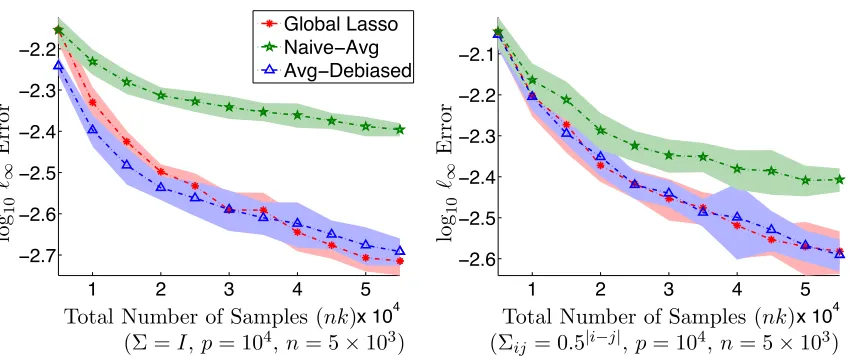
Figure 1: The estimation error (in`∞norm) of the averaged debiased lasso estimator versus
that of the centralized lasso when the predictors are Gaussian. In both settings, the estimation error of the averaged debiased estimator is comparable to that of the centralized lasso, while that of the naive averaged lasso is much worse.
3. kβ˜ht−β∗k1 .P s20logp
N
12
+s0maxj∈[p]sjlogp
n .
Assuming s0 ∼ smax, Theorem 22 shows whenm . s2n 0logp
, the variance term is domi-nant, so the convergence rates simplify to
1. kβ˜ht−β∗k∞.P logNp
12
,
2. kβ˜ht−β∗k2 .P s0logp
N
12
,
3. kβ˜ht−β∗k1 .P s
2 0logp
N
12
.
6. Simulations
We validate our theoretical results with simulations. First, we study the estimation error of the averaged debiased lasso in `∞ norm. To focus on the effect of averaging, we grow
the number of machines m linearly with the (total) sample size N. In other words, we fix the sample size per machine n and grow the total sample size N by adding machines. The tuning parameters were set to their oracle values stated in the Theorem 12. Figure 1 compares the estimation error (in `∞ norm) of the averaged debiased lasso estimator with
that of the centralized lasso. We see the estimation error of the averaged debiased lasso estimator is comparable to that of the centralized lasso, while that of the naive averaged lasso is much worse.
5 10 15 20 −2.8
−2.7 −2.6 −2.5 −2.4 −2.3 −2.2
10 20 30 40 50
−2.6 −2.5 −2.4 −2.3 −2.2 −2.1 −2
Global Lasso Naive−Avg Avg−Debiased
Number of Machines (k) Number of Machines (k)
(Σ =I,p= 104,nk = 2×10⁵) (Σ
ij = 0.5|i−j|,p= 104,nk= 2×10⁵)
log
10
`∞
Error
log
10
`∞
Error
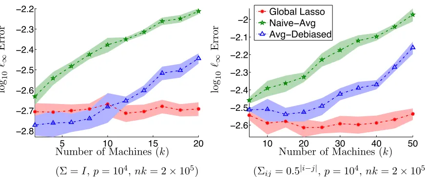
Figure 2: The estimation error (in `∞ norm) of the averaged estimator as the number of
machineskvary. When the number of machines is small, the error is comparable to that of the centralized lasso. However, when the number of machines exceeds a certain threshold, the bias term (which grows linearly in k) is dominant, and the performance of the averaged estimator degrades.
machinesk,we fix the (total) sample size N and vary the number of machines the samples are distributed across. The tuning parameters were again set to the oracle values stated in the Theorem 12. Figure 2 shows how the estimation error (in `∞ norm) of the averaged
estimator grows as the number of machines grows. When the number of machines is small, the estimation error of the averaged estimator is comparable to that of the centralized lasso. However, when the number of machines exceeds a certain threshold, the estimation error grows with the number of machines. This transition occurs when slogn p & logNp12
,
or equivalently, when k & s2Nlogp
12
. The preceding observation is consistent with the prediction of Lemma 10: when the number of machines exceeds a certain threshold, the bias term of order slogn p becomes dominant. Since slogn p ∝k, we expect the error to grow linearly with k, which agrees with the trends in Figure 2.
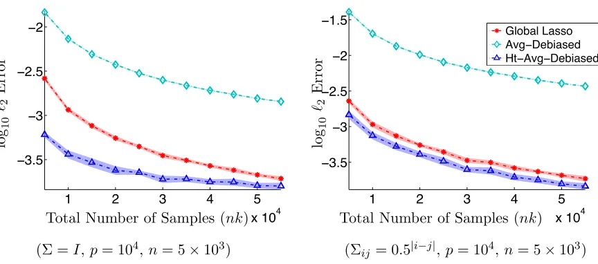
We conduct a third set of simulations to study the effect of thresholding on the estimation error in`2norm. The tuning parameters were set to the oracle values stated in the Theorem 12. Figure 3 compares the estimation error incurred by the averaged estimator with and without thresholding versus that of the centralized lasso. Since the averaged estimator is usually dense, its estimation error (in`2 norm) is large compared to that of the centralized lasso. However, after thresholding, the averaged estimator performs comparably versus the centralized lasso. This demonstrates the importance of the thresholding step to achieve low `2 error.
1 2 3 4 5
x 104
−3.5 −3 −2.5 −2
1 2 3 4 5
x 104
−3.5
−3
−2.5
−2
−1.5
Global Lasso Avg−Debiased Ht−Avg−Debiased
Total Number of Samples (nk) Total Number of Samples (nk)
(Σ =I,p= 104,n= 5×10³) (Σij = 0.5|i−j|,p= 104,n= 5×10³)
log
10
`2
Error
log
10
`2
Error
Figure 3: The estimation error (in `2 norm) of the averaged estimator with and without thresholding versus that of the centralized lasso when the predictors are Gaus-sian. In both settings, thresholding reduces the estimation error by order(s) of magnitude. Although the estimation error of the averaged estimator is large compared to that of the centralized lasso, the thresholded averaged estimator performs comparably, or even better than, the centralized lasso.
λ=σ√2 logp. The parameter λcan be chosen independently of σ, if we replace the lasso with the sqrt-lasso Belloni et al. (2011); all of the same theoretical guarantees still apply, since the sqrt-lasso has the same consistency guarantees. For generalized linear models, the oracle choice of λdepends on known quantities Negahban et al. (2012).
7. Summary and discussion
We devised a communication-efficient approach to distributed sparse regression in the high-dimensional setting. The key idea is first “debiasing” local lasso estimators, and then averaging the debiased estimators. We show that as long as the data is not split across too many machines, the averaged estimator achieves the convergence rate of the centralized lasso estimator. In the appendix, we show that by foregoing consistency in the `∞ norm,
it is possible to further reduce the sample complexity of the averaged estimator to that of the centralized lasso estimator. Further, the distributed approach to debiasing extends readily to other`1 regularized M-estimators. In concurrent work, the approach of averaging debiased M-estimators was proposed by Battey et al. (2015) for high-dimensional inference.
7.1 Communication and Computational complexity
In recent years, there has a been a flurry of work on establishing communication lower bounds for mean estimation in the Gaussian distribution. In other words, they establish the minimum communication C needed to obtain `22 risk R , where kβˆ−β∗k2
regression, since they do not impose sparsity on the mean. In Braverman et al. (2015), the authors established that to obtain risk R ≤ slogNp at least Ω mmin(logpn,p) bits of com-munication is required. Our approach communicates ˜O(mp) bits to achieve risk of slogNp, so is communication-optimal when p . n. To our knowledge, lowest known communica-tion complexity for solving the lasso is at least mpσσmax(Σ)min(Σ) log1, for any desired accuracy &
q
slogp
n (Agarwal et al., 2012). This communication cost is larger than our algorithm
by a multiplicative factor of σσmax(Σ)min(Σ)log1, which is substantially larger when the problem is poorly conditioned.
In light of the fact that our approach is essentially optimal in terms of communication cost, we turn to the computational complexity of our method. The most intensive step of our approach is the computation of ˆΘ. To compute one row of ˆΘ requires solving an optimization problem whose cost is equivalent to a lasso in dimension p with n samples. For the purpose of comparison, let us assume that the lasso solver performs T iterations. Thus the complexity of solving a lasso in dimension p with n samples is O(npT). In the simple approach of Section 2 where each machine computes its own ˆΘ, the parallel runtime isO(np2T). However using the approach of Section 3, each machine is only computingp/m rows of ˆΘ. This brings down the parallel runtime to O(npm2T). In comparison, the cost of solving the lasso using a state-of-art optimization method such as Agarwal et al. (2012) has parallel runtime O(npT), so our computational cost is larger by a factor of O(mp). It is reasonable to think of mp as a constant, since as the number of variables p increases the dataset sizes increases and we will be forced to use a larger cluster sizem due to memory constraints on a single machine. Although our computational complexity is larger in the distributed setting, the dominant factor is often bottlenecked by the communication and latency limitations, rather than local computation.
Appendix A. Proofs of Lemmas
Proof [Proof of Lemma 2] Letzi = Σ−
1
2xi.The generalized coherence between X and Σ−1 is given by
|||Σ−1Σˆ−I|||∞=|||
1 n
n
X
i=1
(Σ−12zi)(Σ 1
2zi)T −I|||∞,
where |||X|||∞ is the maximum entry of aX. Each entry of n1Pni=1(Σ−
1 2zi)(Σ
1
2zi)T −I is a sum of independent subexponential random variables. Their subexponential norms are bounded by
k(Σ−12zi)j(Σ 1
2zi)k−1{j=k}kψ
1 ≤2k(Σ
−1 2zi)j(Σ
1 2zi)kkψ
1,
where kXkψ
1 and kYkψ2 are the sub-exponential and sub-Gaussian norms of the random variables X and Y. Recall for any two subgaussian random variablesX, Y, we have
kXYkψ
1 ≤2kXkψ2kYkψ2. Thus
k(Σ−12zi)j(Σ 1
2zi)k−δj,kkψ
1 ≤4k(Σ
−1 2zi)jkψ
2k(Σ 1 2zi)kkψ
2 ≤4 √
whereσx=kzikψ2.By a Bernstein-type inequality, Pr 1 n n X i=1
(Σ−12zi)j(Σ 1
2zi)k−δj,k ≥t
≤2e−c1min{
nt2
˜
σ4x, nt
˜
σx2
}
,
where c1 > 0 is a universal constant and ˜σx2 := 4
√
κσx2. Since ˜σx4n > logp, we set t = 2˜σ2
x √ c1 logp n 12 to obtain
Pr1 n
n
X
i=1
(Σ−12zi)j(Σ 1
2zi)k−δj,k ≥ 2˜σ 2 x √ c1 logp n 12
≤2p−4.
We obtain the stated result by taking a union bound over thep2entries ofn1 Pn i=1(Σ
−1 2zi)(Σ
1 2zi)T− I.
Proof [Proof of Lemma 5] By Vershynin (2010), Proposition 5.10,
Pr
1
n|x
T j|> t
≤eexp
− c2n 2t2 σ2
ykxTjk22
≤eexp
− c2n 2t2 σ2
ymaxj∈[p]Σˆj,j
.
We take a union bound over thep components of 1nXTto obtain
Pr
1
nkX
Tk
∞> t
≤eexp
− c2n 2t2 σ2
ymaxj∈[p]Σˆj,j
+ logp
.
We set t= maxj∈[p]Σˆ 1 2
j,jσy 3 logc2np
12
to obtain the desired conclusion.
Proof [Proof of Lemma 7] We start by substituting the linear model into (1):
ˆ
βd= ˆβ+ 1 n
ˆ
ΘXT(y−Xβˆ) =β∗+ ˆΘ ˆΣ(β∗−βˆ) + 1 n
ˆ ΘXT.
By adding and subtracting ˆ∆ =β∗−β,ˆ we obtain
ˆ
βd=β∗+ 1 n
ˆ
ΘXT(y−Xβˆ) =β∗+ ( ˆΘ ˆΣ−I)(β∗−βˆ) + 1 n
ˆ ΘXT.
We obtain the expression of ˆβd by setting ˆ∆.
To showk∆kˆ ∞≤ 3µδsλ,we apply H¨older’s inequality to each component of ˆ∆ to obtain
Proof [Proof of Lemma 10] By Lemma 7,
¯
β−β∗= 1 N
m
X
k=1 ˆ
ΘkXkTk+
1 m m X k=1 ˆ ∆k.
We take norms to obtain
kβ¯−β∗k∞≤ 1 N m X k=1 ˆ ΘkXkTk
∞+ 1 m m X k=1
k∆ˆkk∞.
We focus on bounding the first term. Let aT j := eTj
ˆ
Θ1X1T . . . ΘˆmXmT
. By Vershynin (2010), Proposition 5.10,
Pr 1 Na T j > t
≤eexp
−c2N 2t2 kajk22σy2
for some universal constantc2 >0.Further, kajk22 =
m
X
k=1
kXkΘˆTkejk22 =n
m
X
k=1 ˆ ΘkΣˆkΘˆTk
j,j≤cΩN,
wherecΩ := maxj∈[p],k∈[m] ΘˆkΣˆkΘˆTk
j,j.By a union bound overj∈[p],
Pr
maxj∈[p]
1 Na T j > t
≤eexp
−c2N t 2 cΩσ2y
+ logp
.
We set t=σy 2cΩc2logN p
12
to deduce
Prmaxj∈[p]
N1aTj
≥σy 2cΩclogp
2N
12
≤ep−1.
We turn our attention to bounding the second term. By Lemma 5 and a union bound overj∈[p], when we set
λ1 =· · ·=λm =λ:= maxj∈[p],k∈[m](( ˆΣk
j,j)
1 2σy
3 logp
c2n
12
,
we have n1kXkTk∞ ≤ λ for any k ∈ [m] with probability at least 1− emp2 ≥ 1−ep−1. By Lemma 7, when
1. {Σˆk}k∈[m] satisfy the RE condition onC(supp(β∗)) with constant µl,
2. {( ˆΣk,Θˆk)}k∈[m] have generalized incoherence cGC lognp
12
,
the second term is at most 3
√
3
√
c2
cGCcΣ
µl σy
slogp
n . We put the pieces together to obtain
kβ¯−β∗k∞≤σy
2cΩlogp
c2N
1 2 +3 √ 3 √ c2 cGCcΣ
µl
σy
Proof [Proof of Lemma 10] We start with the conclusion of Lemma 10:
kβ¯−β∗k∞≤σy
2cΩlogp
c2N
12
+3 √
3 √
c2 cGCcΣ
µl
σy
slogp n .
First, we show that the two constantscΩ= maxj∈[p], k∈[m]( ˆΘkΣˆkΘˆkT)j,jandcΣ := maxj∈[p],k∈[m](( ˆΣk)j,j)
1 2 are bounded with high probability.
Lemma 23 Under (A1),
Pr maxj∈[p]Σ−j1ΣΣˆ
−1
j >2 maxj∈[p]Σ−j,j1
≤2pe−c1min{
n σx2,
n σx}
for some universal constant c1 >0. Proof [Proof of Lemma 23] We express
Σj,−·1ΣΣˆ −j,·1 = Σ−j,·1ΣΣˆ −j,·1−Σ−j,j1+ Σ−j,j1 = 1 n
n
X
i=1
(xTi Σ−·,j1)2−Σ−j,j1+ Σ−j,j1.
Since the subgaussian norm ofzi= Σ−
1
2xiisσx, xT
i Σ
−1
·,j is also subgaussian with subgaussian
norm bounded by
kxTi Σ−·,j1kψ2 ≤ kzikψ2kΣ
−1 2
·,j k2≤σx(Σ
−1
j,j)
1 2.
We recognize 1nPn
i=1(xTi Σ
−1
·,j)2−Σ
−1
j,j as a sum of i.i.d. subexponential random variables
with subexponential norm bounded by
k(xTi Σ−·,j1)2−Σ−j,j1kψ1 ≤2k(xiTΣ−·,j1)2kψ1 ≤4kxTi Σ−·,j1k2
ψ2 ≤4σ 2
xΣ−j,j1.
By Vershynin (2010), Proposition 5.16, we have
Pr
1
n
n
X
i=1
(xTi Σ·−,j1)2−Σ−j,j1 > t
≤2e
−c1min{ nt 2 16σ2x(Σ−j,j1)2,
nt
4σxΣ−j,j1}
for some absolute constant c1>0.Fort= Σ−j,j1,the bound simplifies to
Pr1 n
n
X
i=1
(xTi Σ−·,j1)2−Σj,j−1 >Σ−j,j1≤2e−c1min{
n
16σx2, n
4σx}.
We take a union bound overj∈[p] to obtain the stated result.
Since we form {Θˆk}k∈[m] by (2),
( ˆΘkΣˆkΘˆTk)j,j≤maxj∈[p](Σ−1ΣˆkΣ−1))j,j.
Lemma 23 implies
maxj∈[p](Σ−1ΣˆkΣ−1))j,j ≤2 maxj∈[p]Σ−j,j1 for each k∈[m]
with probability at least 1−2pe−c1min{
n σ2x,
Lemma 24 Under (A1),
Pr(maxj∈[p]( ˆΣj,j)
1 2 >
√
2 maxj∈[p](Σj,j)
1
2)≤2pe
−c1min{ n 16σ2x,
n
4σx}
for some universal constant c1 >0.
We put the pieces together to obtain the stated result:
1. By Lemma 23 (and a union bound over k∈[m]),
Pr(cΩ ≥2 maxjΣ−j,j1)≤2mpe
−c1min{n
σ2x, n σx}.
Since m≤p,when n > c3
1max{σ 2
x, σx}logp,
Pr cΩ<2 max
j Σ
−1
j,j
≥1−2p−1.
2. By Lemma 24 (and a union bound over k∈[m]),
Pr(cΣ < √
2 maxj∈[p](Σj,j)
1
2)≥1−2mpe
−c1min{ n 16σx2,
n
4σx}.
When n > c3
1max{σ 2
x, σx}logp, the right side is again at most 2p−1.
3. By Lemma 4, as long as
n >max{4000˜sσ2xlog(Cp˜s ),8000σx4logp}, ˆ
Σ1, . . . ,Σˆm all satisfy the RE condition with probability at least
1−2me−
n
4000σ4x ≥1−2p−1.
4. By Lemma 2,
Pr ∩k∈[m]EGC( ˆΣk)
≥1−2p−2. Since m < p,the probability is at least 1−2p−1.
We apply the bounds cΩ ≤2 maxj∈[p]Σ−j,j1, cΣ ≤
√
2 maxj∈[p](Σj,j)
1
2,cGC = √8
c1 √
κσx2, and µl= 12λmin(Σ) to obtain
kβ¯−β∗k∞≤σy
4 max
j∈[p]Σ−j,j1logp
c2N
12
+ 48 √
6 √
c1c2 √
κmaxj∈[p](Σj,j)
1 2 λmin(Σ)
σx2σy
slogp n .
Proof [Proof of Lemma 24] We follow a similar argument as the proof of Lemma 23:
ˆ
Σk;j,j = ˆΣj,j = ˆΣj,j−Σj,j+ Σj,j =
1 n
n
X
i=1
Since the zi = Σ−
1
2xi is subgaussian with subgaussian norm σx, xi,j is also subgaussian with subgaussian norm bounded by
kxi,jkψ2 ≤ kΣ 1 2
j,·zikψ2 ≤σx(Σj,j) 1 2.
We recognize ˆΣj,j −Σj,j = n1Pin=1x2i,j −Σj,j as a sum of i.i.d. subexponential random
variables with subexponential norm bounded by
kΣˆj,j−Σj,jkψ1 ≤2kx 2
i,jkψ1 ≤4kxi,jk 2
ψ2 ≤4σ 2
xΣj,j.
By Vershynin (2010), Proposition 5.16, we have
Pr(|Σˆj,j−Σj,j|> t)≤2e
−c1min{ nt 2 16σx2Σ2
j,j
, nt σxΣj,j}
for some absolute constant c1>0.Fort= Σj,j,the bound simplifies to
Pr(|Σˆj,j−Σj,j|>Σj,j)≤2e
−c1min{ n 16σx2,
n
4σx}.
We take a union bound overj∈[p] to obtain the stated result.
Proof [Proof of Theorem 16] We start by substituting the linear model into (5):
˜ β = 1
m
m
X
k=1 ˆ
βk−Θ ˆˆΣk( ˆβk−β∗) +
1 n
ˆ ΘXkTk
= 1 m
m
X
k=1 ˆ
βk−Θ ˆˆΣk( ˆβk−β∗) +
1 NΘˆX
T.
Subtractingβ∗ and taking norms, we obtain
kβ˜−β∗k∞≤
1 m
m
X
k=1
k(I−Θ ˆˆΣk)( ˆβk−β∗)k∞+
1 N
ˆ
ΘXT∞. (11)
By Vershynin (2010), Proposition 5.16, and Lemma (23), it is possible to show that
1 NΘˆX
T
∞.P
logp
N
1
2 .
We turn our attention to the first term in (11). It’s straightforward to see each term in the sum is bounded by
k(I−Θ ˆˆΣk)( ˆβk−β∗)k∞
≤ k(I−Σ−1Σˆk)( ˆβk−β∗)k∞+k(Σ−1−Θ) ˆˆ Σk( ˆβk−β∗)k∞
≤maxj∈[p]keTj −Σ
−1
j Σˆkk∞kβˆk−β
∗k
1+kΣ−j1−Θˆj,·k1kΣˆk( ˆβk−β∗)k∞.
We put the pieces together to deduce each term isO smaxlogp
n
1. By Lemmas 4, 6, 24,kβˆk−β∗k1.P
√ s0λk.
2. By Lemma 15,kΣ−j1−Θˆj,·k1 .P sj lognp
12
.
3. By the triangle inequality,
kΣˆk( ˆβk−β∗)k∞≤
1 nX
T
k(yk−Xkβˆk)
∞+
1 nX
T kk
∞.
By the optimality conditions of the (local) lasso estimators, the first term isλk, and
it is possible to show, by Lemma 23 and Vershynin (2010), Proposition 5.16, that the
second term isOP lognp
12
.
Since λk lognp
1
2, by a union bound overk∈[m],we obtain
kβ¯−β∗k∞∼OP
logp
N
1
2
+smaxlogp n
,
wheresmax:= max{s0, s1, . . . , sp}.
Proof [Proof of Lemma 18] The result is essentially Javanmard and Montanari (2013b), Theorem 2.3 with ˆΩ = ˆΘ given by (6). Lemma 15 shows that
maxj∈[p]kΘˆj,·−Σ−j1k1 .P sj lognp
12
,
Since maxj∈[p]s 2
jlogp
n ∼o(1), ˆΘ satisfies the conditions of Javanmard and Montanari (2013b),
Theorem 2.3:
k∆ˆkk(∞,c0s0).P
c√s0logp
n for any k∈[m],
The bound is uniform in k ∈[m] by a union bound for suitable parameters λk ∼ lognp
12
.
Proof [Proof of Theorem 19] We start by substituting the linear model into (5):
˜ β = 1
m
m
X
k=1 ˆ ∆k+
1 NΘˆX
T.
Subtractingβ∗ and taking norms, we obtain
kβ˜−β∗k(∞,c0s0)≤ 1 m
m
X
k=1
k∆ˆkk(∞,c0s0)+
1 N
ˆ ΘXT
(∞,c0s0). (12) By Lemma 18, the first (bias) term is of order c
√
s0logp
n . We focus on showing the second
(variance) term is of order logNp12
. Since the (∞, l) norm is non-increasing in l,
1 NΘˆX
T (∞,c0s
0)≤
1 NΘˆX
By Vershynin (2010), Proposition 5.16 and Lemma 23, it is possible to show that
1 NΘˆX
T
∞∼OP
logp
N
12
.
Thus the second term in (12) is of order logNp12
. We put all the pieces together to obtain the stated conclusion.
Proof [Proof of Theorem 20] Since ˜βht−β∗ is 2s0-sparse, kβ˜ht−β∗k2
2 .s0kβ˜ht−β∗k2(∞,c0s0) or, equivalently,
kβ˜ht−β∗k2.√s0kβ˜ht−β∗k(∞,c0s0). By the triangle inequality,
kβ˜ht−β∗k(∞,c0s0)≤ kβ˜ht−β˜k(∞,c0s0)+kβ˜−β∗k(∞,c0s 0) ≤2kβ˜−β∗k(∞,c0s0),
where the second inequality is by the fact that thresholding at t = |β˜|(c0s0) minimizes kβ−β∗k(∞,c0s0) overc0s0-sparse points β. Thus
kβ˜ht−β∗k2 =OP
s0logp
N
1
2
+s0logp n
.
To complete the proof, we observe that the estimation error bound of ˜βht in the `1 norm follows by the fact that ˜βht−β∗ is 2s0-sparse.
References
Alekh Agarwal, Sahand Negahban, Martin J Wainwright, et al. Fast global convergence of gradient methods for high-dimensional statistical recovery. The Annals of Statistics, 40 (5):2452–2482, 2012.
Heather Battey, Jianqing Fan, Han Liu, and Junwei Lu. Splitotic analysis for distributed estimation and hypothesis testing. preprint (personal communication), 2015.
Alexandre Belloni, Victor Chernozhukov, and Christian Hansen. Inference for high-dimensional sparse econometric models. arXiv preprint arXiv:1201.0220, 2011.
Stephen Boyd, Neal Parikh, Eric Chu, Borja Peleato, and Jonathan Eckstein. Distributed optimization and statistical learning via the alternating direction method of multipliers. Foundations and Trends in Machine Learning, 3(1):1–122, 2011.
Peter B¨uhlmann and Sara Van De Geer. Statistics for high-dimensional data: methods, theory and applications. Springer, 2011.
Ofer Dekel, Ran Gilad-Bachrach, Ohad Shamir, and Lin Xiao. Optimal distributed online prediction using mini-batches.The Journal of Machine Learning Research, 13(1):165–202, 2012.
John C Duchi, Alekh Agarwal, and Martin J Wainwright. Dual averaging for distributed optimization: convergence analysis and network scaling. Automatic Control, IEEE Trans-actions on, 57(3):592–606, 2012.
John C Duchi, Michael I Jordan, Martin J Wainwright, and Yuchen Zhang. Optimality guarantees for distributed statistical estimation. arXiv preprint arXiv:1405.0782, 2014.
Ankit Garg, Tengyu Ma, and Huy L Nguyen. Lower bound for high-dimensional statistical learning problem via direct-sum theorem. arXiv preprint arXiv:1405.1665, 2014.
Trevor Hastie, Robert Tibshirani, and Martin Wainwright.Statistical learning with sparsity: the lasso and its generalizations. CRC Press, 2015.
Adel Javanmard and Andrea Montanari. Confidence intervals and hypothesis testing for high-dimensional regression. arXiv preprint arXiv:1306.3171, 2013a.
Adel Javanmard and Andrea Montanari. Nearly optimal sample size in hypothesis testing for high-dimensional regression. arXiv preprint arXiv:1311.0274, 2013b.
Ryan Mcdonald, Mehryar Mohri, Nathan Silberman, Dan Walker, and Gideon S Mann. Efficient large-scale distributed training of conditional maximum entropy models. In Advances in Neural Information Processing Systems, pages 1231–1239, 2009.
Sahand N Negahban, Pradeep Ravikumar, Martin J Wainwright, and Bin Yu. A unified framework for high-dimensional analysis of m-estimators with decomposable regularizers. Statistical Science, 27(4):538–557, 2012.
Garvesh Raskutti, Martin J Wainwright, and Bin Yu. Restricted eigenvalue properties for correlated gaussian designs. J. Mach. Learn. Res., 11:2241–2259, 2010.
Jonathan Rosenblatt and Boaz Nadler. On the optimality of averaging in distributed sta-tistical learning. arXiv preprint arXiv:1407.2724, 2014.
Mark Rudelson and Shuheng Zhou. Reconstruction from anisotropic random measurements. Information Theory, IEEE Transactions on, 59(6):3434–3447, 2013.
Sara van de Geer, Peter B¨uhlmann, Ya’acov Ritov, and Ruben Dezeure. On asymptoti-cally optimal confidence regions and tests for high-dimensional models. arXiv preprint arXiv:1303.0518, 2013.
Cun-Hui Zhang and Stephanie S Zhang. Confidence intervals for low dimensional parameters in high dimensional linear models. Journal of the Royal Statistical Society: Series B (Statistical Methodology), 76(1):217–242, 2014.
Yuchen Zhang, John C Duchi, and Martin J Wainwright. Communication-efficient algo-rithms for statistical optimization. Journal of Machine Learning Research, 14:3321–3363, 2013.