Numerical Solution of Flow and Heat Transfer
of Second Order Fluid over a Stretching Sheet
Dr. V. Dhanalaxmi
##Associate Professor of Mathematics, University College of Technology, Osmania University, Hyderabad
Telangana State, India 500 007
Abstract: An analysis is carried out to study the flow and heat transfer characteristics in the laminar boundary layer flow of a second order fluid over a linearly stretching sheet with internal heat generation or absorption. The governing partial differential equations are converted into ordinary differential equations by a similarity transformation. A numerical method, quasilinearization technique is used to study velocity and temperature profiles of the fluid. Heat transfer analysis is carried out for two types of thermal boundary conditions namely, (i) Prescribed Surface temperature (PST) and (ii) Prescribed wall Heat Flux (PHF). The effects of various parameters on flow and heat transfer are presented through graphs and discussed.
Keywords: visco-elasticity, stretching sheet, Prandtl number, boundary layer, heat transfer, second order fluid.
I. INTRODUCTION
In many engineering processes, boundary layer behaviour occurs for a flow over a moving continuous solid surface. Manufacturing processes that involve extrusion of a material and heat-treated materials that travel between feed and wind-up rollers or on conveyer belts are examples that exhibit the characteristics of flow over a moving continuous surface. Sakiadis [1] initiated the study of these applications by considering the boundary layer flow over a continuous solid surface moving with constant speed. Erickson et al [2] extended this problem to the case in which the transverse velocity at the moving surface is non zero, with heat and mass transfer in the boundary layer being taken into account.
The above investigations have a definite bearing on the problem of a polymer sheet extruded continuously from a die. It is usually assumed that the sheet is inextensible, but situations may arise in the polymer industry in which it is necessary to deal with a stretching plastic sheet, as noted by Crane [3]. Danberg and Fansler [4] investigated the non-similar solution for the flow in the boundary layer past a wall that is stretched with a velocity proportional to the distance along the wall.
Dutta, Roy and Gupta [5] have analysed the temperature distribution in the flow over a stretching sheet with uniform wall heat flux. Vajravelu and Rollins [6] investigated the heat transfer
characteristics in a visco-elastic fluid over a continuous impermeable, linearly stretching sheet with PST and PHF cases. They studied the heat transfer characteristics in fluid initially at rest and at uniform temperature. As there is an appreciable temperature difference between the surface and the ambient fluid, one needs to consider the temperature dependent heat sources or sinks which may exert strong influence on the heat transfer characteristics.
Foraboschi and Federico [7] studied heat transfer in a laminar flow of non-Newtonian heat generation fluids. Vajravelu and Hadjinicolaou [8] have studied the heat transfer characteristics in a viscous fluid over a stretching sheet with viscous dissipation and internal heat generation. Vajravelu and Roper [9] analysed heat transfer characteristics in a second grade fluid over stretching sheet with viscous dissipation, internal heat generation, and work due to deformation. Rollins and Vajravelu [10] studied flow and heat transfer characteristics in a second order fluid over a stretching sheet. In many of these studies, analytical solutions for flow and heat transfer are obtained for different wall temperature.
Motivated by the above studies, present paper gives a numerical solution for flow and heat transfer of an incompressible second order fluid past stretching sheet with internal heat generation. A numerical approach, Quasilinearization technique is used to study flow and heat transfer characteristics of the fluid. This approach is easily adoptable and it is observed that results are in good agreement with the available literature. The effects of various parameters on flow and heat transfer are analysed through numerical calculations.
II. MATHEMATICAL FORMULATION
Following the postulates of gradually fading memory, Coleman and Noll [11] derived the constitutive equation of second-order fluid flow in the form
2 1 2 2 1
1
A
A
A
pI
T
(1)Where T is the Cauchy stress tensor, -pI is the spherical stress due to constraint of incompressibility, µ is the dynamics viscosity, α1, α2 are the material constants and A1 and A2 are the first two Rivlin-Ericksen tensors [12] defined as
T
v
grad
v
grad
1 1
1
2
A
(
grad
v
)
(
grad
v
)
A
dt
dA
A
T (3)Here, ν denotes the velocity field and d/dt is the material time derivative. If the fluid of second grade modeled by (1) is to be compatible with thermodynamics and is to satisfy the Clausius-Duhem inequality for all motions and the assumption that the specific Helmholtz free energy of the fluid is a minimum when it is locally at rest, Dunn and Fosdick [13] found that the material moduli must satisfy
0
,
0
,
0
1
1
2
(4)But later on Fosdick and Rajagopal [14] have reported, by using the data reduction from experiments, that in the case of a second order fluid the material constants µ,α1, α2 should satisfy the relation
0
,
0
,
0
1
1
2
(5)They also reported that the fluids modeled by (1) with the relationship (5) exhibit some anomalous behavior. A critical review on this controversial issue can be found in the work of Dunn and Rajagopal [15]. Second-order fluid, obeying model equation (1) with α1<α2, α1<0 although exhibits some undesirable instability characteristics, its approximations are valid at low shear rate. Now in literature the fluid satisfying the model equation (1) with α1<0 is termed as second-order fluid and with α1>0 is termed as second grade fluid.
A laminar steady flow of an incompressible viscoelastic (Walters’ liquid B model) fluid over a wall coinciding with the plane y = 0 is considered, the flow being confined to y > 0. Two equal and opposite forces are applied along the x-axis, so that a sheet is stretched with a velocity proportional to the distance from the origin. The resulting motion of the quiescent fluid is thus caused solely by the moving surface. The flow satisfies the rheological equation of state derived by Beard and Walters [16]. The steady two-dimensional boundary layer equations for this fluid, in the usual form are
0
y
v
x
u
(6)
3 3
2 2
2 2
0 2 2
y
u
v
y
v
y
u
y
u
u
x
k
y
u
y
v
v
x
u
u
(7)
0
,
0
k
where
Where µ and ν are the velocity components along the x and y directions respectively, ν is the kinematic viscosity k0=-α1/ρ is the co-efficient of elasticity, and ρ is the density. Hence, in the case of second order fluid flow, k0takes positive value, as α1takes negative value and other quantities have their usual meanings. In deriving the equation (7), it is assumed
magnitude as that of the shear stress, in addition to usual boundary layer approximations.
The boundary conditions for the velocity field are
y
as
y
u
u
b
y
at
v
bx
u
u
w0
,
0
0
,
0
0
,
(8)
The condition
u
/
y
0
as
y
is the augmented condition, since the flow is in an unbounded domain, which has been discussed by Rajgopal [17]. In this case, the flow is caused solely by the stretching of the sheet, since the free stream velocity is zero.Defining new variables:
v
b
f
b
y
bxf
u
,
,
/
(9)
where fƞ (ƞ) denotes differentiation with respect to η.
Clearly u and v defined above satisfy the continuity
equation (6), and the equation (7) reduces to
2
1 2
2
ff
f
k
f
f
ff
f
f
(10)
Where k1=k0b/ν, is the visco-elastic parameter. The boundary conditions (8) become
0
0
,
f
0
1
f
(11a)
f
as
f
0
,
0
(11b)III. HEAT TRANSFER ANALYSIS
The governing boundary layer equation with internal heat generation or absorption is given by
T T Q y
T k y T v x T u
Cp 2
2
(12)Where k is the thermal diffusivity and cp is the specific heat of a fluid at constant pressure and Q is the volumetric rate of heat generation.
Since there is an appreciable temperature difference between the surface and the ambient fluid, temperature dependent heat sources or sinks exert strong influence on the heat transfer characteristics so above equation (12) includes internal heat generation or absorption.
Here the thermal boundary condition depends on the type of heating process under consideration. Heat transfer analysis is carried out for two types of thermal boundary conditions namely, (i) Prescribed Surface temperature (PST) and (ii) Prescribed wall Heat Flux (PHF),which are given below.
A.Prescribed Surface Temperature (PST case)
2
l
x
A
T
T
T
w at y=0 (13a)
T
as
y
T
(13b)Here l is the characteristic length. Define non-dimensional temperature as
T
T
T
T
w
(14)Using (14), equation (12) reduces to
2
Pr
0
Pr
f
f
(15)Where Pr = µcp / k, Prandtl number, α =Q/(bρcp), heat source/sink parameter.
With boundary conditions
0
1
,
0
(16)B. Prescribed surface Heat Flux (PHF Case)
Prescribed power law surface heat flux (PHF), where surface issubjected to a power law heat flux qw on the wall surface is considered to be a quadratic power of x in the form
2
l
x
D
q
y
T
k
w at y = 0 (17)T T as y
Where D is a constant, k is the thermal conductivity.
Define a dimensionless, scaled temperature as
T
T
T
T
g
w
(18)where
b
l
x
k
D
T
T
w
2
Using (18), equation (12) reduces to
2
Pr
0
Pr
fg
f
g
g
(19)Boundary conditions are:
as
g
at
g
0
0
1
(20)
IV. NUMERICAL SOLUTION OF THE PROBLEM
The flow equation (10) coupled with energy equation (15) or (19) constitute a set of highly nonlinear differential equations in each thermal boundary condition. So obtaining closed form solution for this set is cumbersome and time consuming. Hence quasilinearization method, given by Bellman & Kalaba [18] is used to solve this system. This method is quadratically convergent, starting from the initial guess value and the solution is valid for a large range of parameters. Even when the required number of initial conditions is not given, this method converges very fast.
For convenience equations (10), (15) and (19) are rearranged as
2
1 1
2
1
2
1
f
k
f
f
k
f
f
f
f
f
k
f
iv
(21)
Pr
f
Pr
2
f
(PST case) (22a)
f
g
g
f
g
Pr
2
Pr
(PHF case) (22b)
In order to implement the quasilinearization method, the equations (21) and (22) are converted to a system of first order differential equations by substituting
f
,
f
,
f
,
f
,
,
x
1,
x
2,
x
3,
x
4,
x
5,
x
6
(PST case) (OR)
f
,
f
,
f
,
f
,
g
,
g
x
1,
x
2,
x
3,
x
4,
x
5,
x
6
(PHF case)
Then equations (21) and (22) reduce to:
2 1
x
d
dx
3 2
x
d
dx
4 3
x
d
dx
2
3 1 4 2 1 4 3 1 2 2 1 1 4
2
1
x
k
x
x
k
x
x
x
x
x
k
d
dx
5
x
6d
dx
2
56 1 6
Pr
2
Pr
x
x
x
x
d
dx
(23)(PST &PHF cases)
Using Quasilinearization technique, the system (23) can be linearized as
4 1
1 3
1 3 1 2
1 2 1 1
r r
r r
r r
x
d
dx
x
d
dx
x
d
dx
13 3 1 1 1 1 1 2 4 1 2 1 1 1 1 2 3 1 4 2 1 4 2 2 2 1 1 1 4
2
1
2
2
1
2
1
r r r r r r r r r r r r r r r rx
x
k
x
x
k
x
x
k
x
x
k
x
x
k
x
x
k
x
x
x
k
d
dx
r r r r r x k x x x k xk 1 1
4 1 4 2 1 1 1 2 1 1 1 6 1 5
r rx
d
dx
(24)
r r r r
r r r r r r r r r
x
x
x
x
x
x
x
x
x
x
x
x
d
dx
5 2 6 1 1 6 1 1 5 2 1 2 5 1 1 6 1 6Pr
2
Pr
Pr
2
Pr
Pr
2
Pr
The above system of equations (24) is linear in
x
ir1(
i
1
,
2
,...
6
) and general solution can be obtained by using the principle of superposition.The boundary conditions given by (11), (16) and (20)reduce to
PST case:
0
0
,
2 1
0
,1
5 1
0
1
1
1
r r
r
x
x
x
(25a)PHF case:
0
,0
0
,1
6 1
0
1
1 2 1
1
r r
r
x
x
x
(25b)
as
x
x
x
2r10
,
3r10
,
5r10
The initial values are chosen as follows:
For homogeneous solution:
0
0
1
0
0
0
1
h i
x
0
0
0
1
0
0
2
h i
x
(26)
0
0
0
0
0
1
3
h i
x
(PST case)(OR)
0
0
0
0
1
0
3
h i
x
(PHF case)For particular solution:
0
1
0
0
1
0
p i
x
(PST case) (27a) (OR)
0
1
0
0
0
1
p i
x
(PHF case) (27b)The general solution for the system (24) is given by
p i h i h i h i r ix
x
C
x
C
x
C
x
3 2 1 3 2 1 1 (28)where C1, C2, C3 are the unknown constants, which are to be determined by considering the boundary conditions as
. This solution
xir1,i1,2,...6
is then compared with solutionat the previous step
xri 1,2,...6
i and next
iteration is performed, if the convergence has not been achieved or greater accuracy is desired.
V. RESULTS AND DISCUSSIONS
The flow and heat transfer characteristics of an incompressible second order fluid past a stretching sheet are studied for two types of thermal boundary conditions i) Prescribed Surface Temperature (PST) and ii) Prescribed Heat Flux (PHF) with internal heat generation or absorption. The governing boundary layer equations are solved using Quasilinearization Technique. The computational results of flow and heat transfer characteristics for various parameters are presented in graphs and discussed.
Fig.1 (a) and Fig. 1(b) depict the effect of viscoelastic parameter k1 on longitudinal and transverse velocity components. It can be seen that for a fixed value of η, f(ƞ) and f(ƞ) decrease with increasing values of viscoelastic parameter k1. This can be explained by the fact that, as the viscoelastic parameter k1 increases, the boundary layer adheres strongly to the surface, which in turn retards the flow in longitudinal and transverse directions.
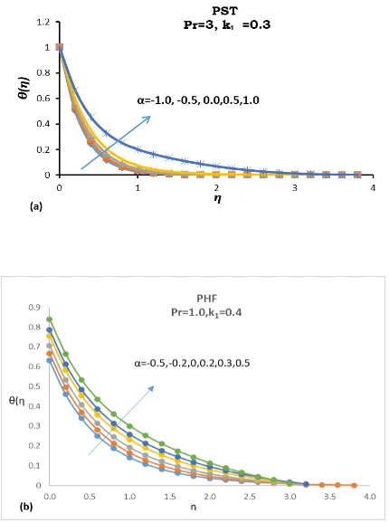
In Fig.2(a) and 2(b), non-dimensional temperature θ(ƞ) is plotted for various values internal heat source/sink parameter (α). It shows that θ(ƞ) increases with increasing values α. This is due to the fact that heat is generated inside the boundary layer for increasing values of heat source/sink parameter (α).
Fig. 3(a) and 3(b) show the effect of Prandtl number (Pr) on non-dimensional temperature θ(ƞ) profiles. Temperature θ(ƞ) decreases with increase in the Prandtl number (Pr), this is consistent with the fact that the thermal boundary layer thickness decreases with increasing values Prandtl number (Pr).
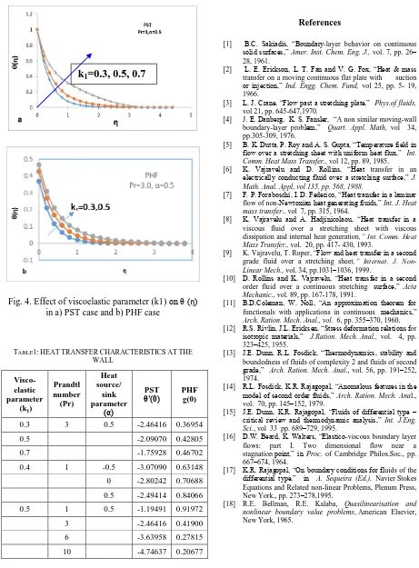
In Fig. 4(a) and 4(b) display the values of temperature θ(ƞ) for different values of viscoelastic parameter (k1). It can be observed that, at a given point η, θ(ƞ) increases with increasing values of k1. This is due to the fact that viscoelastic normal stress gives rise to thickening of thermal boundary layer.
boundary layer are tabulated in Table 1.This reveals that the increase in visco elastic parameter (k1) is to increase the wall temperature gradient θ’(0) in PST case and wall temperature g (0) in PHF case. The increase in value of heat source/sink parameter (α) is to increase both θ’ (0) and g (0). Effect of Prandtl number (Pr) is to decrease the magnitude in both the cases.
From our numerical results, it can be concluded that, temperature of the fluid increases with increasing values of viscoelastic parameter k1. Hence viscoelastic liquids having low viscous dissipation must be chosen. It also increases with increasing values of heat source/sink parameter (α). Hence heat source/sink parameter (α) is better suited for cooling purposes. Temperature of the fluid decreases with increasing values of Prandtl number Pr.
The results of the PHF cases are qualitatively similar to that of the PST case, but quantitatively in the reduced magnitude. The Power Law Heat Flux (PHF) boundary condition is better suited for effective cooling of the stretching sheet.
Fig.1: Effect of viscoelasticity (k1) on (a) transverse velocity component, (b) longitudinal velocity
component
Fig. 2: Effect of heat source/sink parameter (α) on temperature distribution θ (η) in a) PST case b) PHF
case
Fig. 4. Effect of viscoelastic parameter (k1) on θ (η) in a) PST case and b) PHF case
TABLE1:HEATTRANSFERCHARACTERISTICSATTHE WALL
Visco- elastic parameter
(k1)
Prandtl number (Pr)
Heat source/
sink parameter
(α)
PST θ'(0)
PHF g(0)
0.3 3 0.5 -2.46416 0.36954
0.5 -2.09070 0.42805
0.7 -1.75928 0.46702
0.4 1 -0.5 -3.07090 0.63148 0 -2.80242 0.70688 0.5 -2.49414 0.84066 0.5 1 0.5 -1.19491 0.91972
3 -2.46416 0.41900
6 -3.63958 0.27815
10 -4.74637 0.20677
References
[1] B.C. Sakiadis, “Boundary-layer behavior on continuous solid surfaces,” Amer. Inst. Chem. Eng. J., vol. 7, pp. 26– 28, 1961.
[2] L. E. Erickson, L. T. Fan and V. G. Fox, “Heat & mass transfer on a moving continuous flat plate with suction or injection,” Ind. Engg. Chem. Fund, vol 25, pp. 5- 19, 1966.
[3] L. J. Crane, “Flow past a stretching plate,” Phys.of fluids,
vol 21, pp. 645-647,1970.
[4] J. E. Danberg, K. S. Fansler, “A non similar moving-wall boundary-layer problem,” Quart. Appl. Math, vol 34, pp.305-309, 1976.
[5] B. K. Dutta, P. Roy and A. S. Gupta, “Temperature field in flow over a stretching sheet with uniform heat flux,” Int. Comm. Heat Mass Transfer., vol 12, pp. 89, 1985. [6] K. Vajravelu and D. Rollins, “Heat transfer in an
electrically conducting fluid over a stretching surface,” J. Math. Anal. Appl, vol 135, pp. 568, 1988.
[7] F. P. Foraboschi, I. D. Federico, “Heat transfer in a laminar flow of non-Newtonian heat generating fluids,” Int. J. Heat mass transfer., vol 7, pp. 315, 1964.
[8] K. Vajravelu and A. Hadjinicolaou, “Heat transfer in a viscous fluid over a stretching sheet with viscous dissipation and internal heat generation,” Int. Comm. Heat
Mass Transfer., vol. 20, pp. 417- 430, 1993.
[9] K. Vajravelu, T. Roper, “Flow and heat transfer in a second grade fluid over a stretching sheet,” Internat. J. Non-Linear Mech., vol. 34, pp.1031–1036, 1999.
[10] D. Rollins and K. Vajravelu, “Heat transfer in a second order fluid over a continuous stretching surface,” Acta Mechanic., vol. 89, pp. 167-178, 1991.
[11] B.D.Coleman, W. Noll, “An approximation theorem for functionals with applications in continuous mechanics,”
Arch. Ration. Mech. Anal., vol. 6, pp. 355–370, 1960. [12] R.S. Rivlin, J.L. Ericksen, “Stress deformation relations for
isotropic materials,” J.Ration. Mech. Anal., vol. 4, pp. 323–425, 1955.
[13] J.E. Dunn, R.L. Fosdick, “Thermodynamics, stability and boundedness of fluids of complexity 2 and fluids of second grade,” Arch. Ration. Mech. Anal., vol. 56, pp. 191–252, 1974.
[14] R.L. Fosdick, K.R. Rajagopal, “Anomalous features in the model of second order fluids,” Arch. Ration. Mech. Anal., vol. 70, pp. 145–152, 1979.
[15] J.E. Dunn, K.R. Rajagopal, “Fluids of differential type – critical review and thermodynamic analysis,” Int. J.Eng. Sci., vol 33 pp. 689–729, 1995.
[16] D.W. Beard, K. Walters, “Elastico-viscous boundary layer flows: part I. Two dimensional flow near a stagnation point,” in Proc. of Cambridge Philos.Soc., pp. 667–674, 1964.
[17] K.R. Rajagopal, “On boundary conditions for fluids of the differential type,” in A. Sequeira (Ed.), Navier Stokes Equations and Related non-linear Problems, Plenum Press, New York., pp. 273–278,1995.
[18] R.E. Bellman, R.E. Kalaba, Quasilinearisation and nonlinear boundary value problems, American Elsevier, New York, 1965.