232
Copyright © 2018. IJEMR. All Rights Reserved.
Volume-8, Issue-2, April 2018
International Journal of Engineering and Management Research
Page Number: 232-236
DOI:
doi.org/10.31033/ijemr.v8i02.11652
Strong Consistency and Asymptotic Distribution of Estimator for the
Intensity Function Having Form of Periodic Function Multiplied by
Power Function Trend of a Poisson Process
Nina Valentika1, I. Wayan Mangku2 and Windiani Erliana3 1
Student, Department of Mathematics, Bogor Agricultural University, INDONESIA 2,3Lecturer, Department of Mathematics, Bogor Agricultural University, INDONESIA
1Corresponding Author: [email protected]
ABSTRACT
This manuscript discusses the strong consistency and the asymptotic distribution of an estimator for a periodic component of the intensity function having a form of periodic function multiplied by power function trend of a non-homogeneous Poisson process by using a uniform kernel function. It is assumed that the period of the periodic component of intensity function is known. An estimator for the periodic component using only a single realization of a Poisson process observed at a certain interval has been constructed. This estimator has been proved to be strongly consistent if the length of the observation interval indefinitely expands. Computer simulation also showed the asymptotic normality of this estimator.
Keywords— Asymptotic Distribution, Intensity Function, Power Function Trend, Strong Consistency
I.
INTRODUCTION
The stochastic process is a process that describes the events or phenomena relating to the rules of probability. For example, this process can be used to create a model to predict the arrival of a customer to a service center, such as banks, post offices, bookstores, and supermarkets. Based on the time of occurrence, stochastic processes can be divided into two, i.e. the stochastic process with discrete time and stochastic processes with continuous time. In this paper, the discussion focuses only on one form of stochastic processes with continuous time, i.e. the Poisson process periodically.
The periodic Poisson process is a non-homogeneous Poisson process with an intensity function in the form of a periodic function. In the periodic Poisson process, there are two types of intensity functions, i.e. the global intensity function and the local intensity function. The global intensity function in periodic Poisson process states the average rate of the process in an interval of
length towards the infinite, while the local intensity function states the rate of this process at a point.
In general, the intensity function of a phenomenon that is modeled by a stochastic process is unknown, so a method is needed to predict the function. The estimation of the studied intensity function in this paper is the estimation of the local intensity function. Estimation of the local intensity function of a Poisson process at a point was approached by estimating the average number of occurrences of the Poisson process in the time intervals around the point. In order that observational data in different parts of different time intervals can be used to estimate the intensity function at a point, then it is necessary to assume that the intensity function is periodic (cyclic) with a period of the intensity function is known.
One of the benefits of applying the Periodic Poisson process is to create a model of the customer arrival process to the post office. The local intensity function of the process states the rate of arrival of the customer at a given point in time. If the arrival rate of the customer between the previous period and the next period increases according to the power function to the time, then a more appropriate model to use is a periodic Poisson process with a trend component having form of a power function, so that in a long period of time this periodic model requires the intensity function accommodating a trend.
The weak consistency of the intensity function estimator having a form of periodic function multiplied by the trend of power function proposed in [1]. The estimation method used in [1] is a non-parametric method, so the distribution for the estimator intensity function is unknown. Hence, in this paper, a strong consistency was discussed and a simulation was conducted to see the asymptotic distribution of the estimator intensity function.
233
Copyright © 2018. IJEMR. All Rights Reserved.
In this paper, proving strong consistency and tosimulate to see the asymptotic distribution of an estimator for periodic function multiplied by power function trend of a non-homogeneous Poisson process by using a uniform kernel function.The method that will be used to prove the strong convergence of this periodic component estimator is to use the concept of complete convergence and Lemma Borel-Cantelli.
In addition, we also conducted a simulation to verify the asymptotic normality of the studied estimator of the periodic components of the intensity function. The simulation is done by generating the local intensity estimator at the finite observation interval using software R. The method used to generate the realization of the Poisson process is the Monte Carlo method.
Thus, the simulation algorithm performed is as follows:
1. Generate the realization of the periodic Poisson process at the interval of observation and period .
2. Generate the estimator at a given point using the optimal bandwidth .
3. Looking at the asymptotic distribution of the estimator.
In addition, the Distribution Fit Test is done using Mathematica 11.0 software to determine the probability of the normal distribution of the intensity function estimator at a given sample point.
III.
PRIOR APPROACH
In [1], the estimator for the intensity function obtained as the product of a periodic function with the power function trend of a non-homogeneous Poisson process with uniform kernel function has been formulated. In addition, asymptotic approximations to the bias, variance, and mean squared error of this estimator have been established.
Review Construction of The Estimator
Let be a non-homogeneous Poisson process on having (unknown) locally integrable intensity function . It is assumed that the intensity function to be a product of a periodic function with the power function trend, that is, the equation
( ( ( ( holds true for each point , where ( is a periodic function with period (known), is the power function trend with (known), and denotes the slope of the power function trend with . It is not assumed that any (parametric) form of except that it is periodic.
Without loss of generality, the intensity function given in (1) can also be written as
( ( ( ) where ( ( is also a periodic function with period . Hence, for each point and all , with denotes the set of integers, so
( ( By (2) and (3), the problem of estimating at a given point can be reduced to the problem
estimating at a given point [1]. It is assumed throughout that is a Lebesgue point of , that is
∫| ( ( |
(Eg. see [4], p. 107-108), which automatically means that is a Lebesgue point of as well.
The estimator of ( at a given point has been formulated in [1] as follows:
̂ (
∑
(
(
(
with ( denotes the number of occurrence in the interval and be a sequence of positive real numbers converging to zero, that is,
(6)
as . In (5), disebut bandwidth.
Several Lemma which states the statistical properties of the estimator have been established in [1] and [2]as follows:
Lemma 1 (Asymptotic unbiasedness)
Suppose that the intensity function satisfies (2) and is locally integrable. If satisfies assumptions
, then ( ̂ ( ) ( as , provided
is a Lebesgue point of ( . In other words, ̂ ( is the asymptotic unbiased estimator of ( .
The proof of Lemma 1 is referred to [1]
Lemma 2 (Asymptotic approximation to the variance) Suppose that the intensity function satisfies (2) and is locally integrable. If satisfies assumptions
and is a Lebesgue point of ( , then
( ̂ (
{
(
( ( ) (
( (
(
(
) (
( (
( ) (
as with ( (∑ (
).
The proof of Lemma 2 is referred to [1].
Lemma 3 (Asymptotic approximation to the bias) Suppose that the intensity function satisfies (2) and is locally integrable. If satisfies assumptions , , and has a finite second derivative
in s, then
( ̂ ( ) (
(
( (10)
as .
The proof of Lemma 3 is referred to [2].
234
Copyright © 2018. IJEMR. All Rights Reserved.
{
( (
( ( ( )
(
(
( (
( ( ) ( ( )
(
( ( ( ( ( )
⁄
(
with ( (∑ ( ).
The proof of the optimal bandwidth is referred to [2].
IV.
OUR APPROACH
Strong consistency of the estimator is implied by the complete convergence of that estimator. Hence, to prove the strong consistency of the estimator given in (5), then the complete convergence of the estimator needs to be proved. In addition, Lemma 1 and Lemma 2 in [1] are needed for proving the complete convergence of the estimator proposed in [1].
Theorem 1 (Complete Convergence of ̂ ( )
Suppose that the intensity function satisfies (2) and is locally integrable. If , for the case , and for the case , then
̂ ( (
as , provided is a Lebesgue point of . In other words, ̂ ( is complete convergence to ( as
.
Proof of Theorem 1
To prove ̂ ( converges completely to ( , it will be shown that for all ,
∑ (| ̂ ( ( | )
First, the probability in (14) can be written as
(| ̂ ( ̂ ( ̂ ( ( | )
By the triangle inequality, (15) can be written as
(| ̂ ( ̂ ( | | ̂ ( ( |)
By Lemma 1, so that for all , such that
| ̂ ( ( | , (17)
By Lemma 1 and Chebyshev inequality, the probability in (16) is equal to
(| ̂ ( ̂ ( | )
( ̂ ( )
Hence, to prove (14), the following will be sufficient
∑ ( ̂ ( )
By Lemma 2, the variance of ̂ ( is verified
into three cases, i.e. if , , and . The
first case, i.e. if . Since for , then based on (7) in Lemma 2 and series- , the following is obtained
∑ ( ̂ ( )
∑ { (
( ( )}
The second case, i.e. if . Since for
, then based on (8) in Lemma 2 and series-p, the following is obtained
∑ ( ̂ ( )
∑ { ( (
(
(
)}
The third case, i.e. if . Since for , then based on (9) in Lemma 2 and series-p, the following is obtained
∑ ( ̂ ( )
∑ {
( (
( )}
with ( (∑ ( ).
This completes the proof of Theorem 1.
Corollary1 (Strong Consistency)
Suppose that the intensity function satisfies (2) and is locally integrable. If , for the case , and for the case , then
̂ (
→ (
as , provided is a Lebesgue point of . In other words, ̂ ( is a strong consistent estimator of ( .
Proof of Corollary1
To show that ̂ ( is a strong consistent
estimator of ( , it suffices to show that [3], for all ,
( | ̂ ( ( | ) or (23)
( | ̂ ( ( | ) .
(24)
By Theorem 1, we have (14). Suppose that
{| ̂ ( ( | }
then by the Borel-Cantelli Lemma, it is obtained that
( Hence,
(
) ( {| ̂ ( ( | })
This completes the proof of Corollary 1.
Based on Theorem 1 and Corollary 1, then
̂ ( is a strong consistent estimator of ( .
Asymptotic Normality Simulation
235
Copyright © 2018. IJEMR. All Rights Reserved.
observation interval length . The method being usedto generate the realization of the periodic Poisson process is the Monte Carlo Method. This simulation is aimed to verify the asymptotic normality estimator of the studied intensity function periodic component.
The intensity function is being used in this simulation, that is,
( ( ( ))
with ( ( )) is the periodic component and is the power function trend component. The chosen parameter for the intensity function in (25) is ,
, , and . Hence, the intensity function in (25) becomes
( ( ( ))
Graphic illustration intensity function of ( in (26) and its estimation value is presented in Figure 1 and Figure 2.
Figure 1: The intensity function ( and itsestimation value in the interval of observation
Figure 2: The intensity function ( and its estimation value in the interval of observation
Based on Figure 1 and Figure 2, it can be concluded that the estimation value of the intensity function ( at the observation interval is close to the intensity function real value compared to the observation interval . So that the longer the observation interval length being used, then the better estimation will be obtained.
Asymptotic distribution of the estimator is distribution being used to approach a finite sample distribution. This simulation will show that the studied estimator asymptotic distribution is close to normal distribution. To see the asymptotic distribution, first we will estimate the studied intensity function. In estimating
the intensity function is being used two sample points i.e.
(presenting ( that is small) and (presenting ( that is big). The bandwidth being used to estimating the intensity function is the optimal bandwidth for the case proposed in [2].The optimal bandwidth is
( (
( ( ( )
(
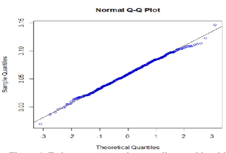
The result of asymptotic normality simulation for ̂ ( is presented in Figure 3 and Figure 4.
Figure 3: Estimator asymptotic normalitygraphic with realization in the interval point (
and
Figure 4: Estimator asymptotic normality graphic with realization in the interval point (
and
Based on Figure 3 and Figure 4, the studied estimator intensity function is close to normality line. Besides, the result of Distribution Fit Test using software Mathematica 11.0 showed that the estimator at point
and normally distributed with the probability of 0.809339 and 0.844338, respectively. Hence, the studied estimator asymptotic distribution is indicated to be closed to the normal distribution.
V.
CONCLUSION
236
Copyright © 2018. IJEMR. All Rights Reserved.
indication that the asymptotic distribution of the estimatorwhich proposed in [1] is approaching thenormal distribution.
REFERENCES
[1] Lewis, P. A. W., & Shedler, G. S. (1979). Simulation of nonhomogeneous poisson process by thinning. Naval Research Logistics, 26(3), 403–413.
[2] Arkin, B. L. & Leemis, L. M. (2000). Nonparametric estimation of the cumulative intensity function for a nonhomogeneous poisson process from overlapping realizations. Management Science, 46(7), 989–998. [3] Grimmett GR & Stirzaker DR. (1992). Probability and random processes. (2nd ed.). Oxford (GB): Clarendon Press.